introduction | linear programming | convex optimization | integer programming | overdetermined problems | underdetermined problems | duality
glpk | matlab/cvx | r/lpsolve | python/cvxopt | excel
introduction
A general form of an optimization problem is to minimize g(x) subject to
(1)where x is a n-dimensional real vector and g and fᵢ are real-valued.
g is the objective function. The components of x are the decision variables. The fᵢ(x) ≤ bᵢ are the constraints.
The maximum of g is the minimum of -g, so a maximization problem can be recast as a minimization problem. The value of the decision variables at the optimum is the same, but the sign of the value of the objective function at the optimum is reversed.
A constraint of the form h(x) = c can be replaced by two constraints of the form h₁(x) ≤ c and h₂(x) ≥ c without changing the meaning of the problem. Moreover, a constraint of the form h(x) ≥ c can be replaced with the equivalent constaint -h(x) ≤ -c.
linear programming
If the objective function g = ∑cᵢ xᵢ and the inequality constraint functions fᵢ = ∑ aᵢⱼ xⱼ are linear, the problem is a linear optimization problem, also called a linear program.
A general form for a linear program is to minimize cTx subject to A x ≤ b and x ≥ 0. Here c and x are vectors with length equal to the number of decision variables. b is a vector with length equal to the number of constraints, and A is a matrix with row count equal to the number of constraints and column count equal to the number of decision variables.
The constraint x ≥ 0 can be imposed without loss of generality by replacing each decision variable xᵢ with xᵢ+ - xᵢ-, where xᵢ+ ≥ 0 and xᵢ- ≥ 0.
convex optimization
integer programming
overdetermined problems
underdetermined problems
duality
The dual problem of maximizing cTx subject to Ax ≤ b and x ≥ 0 is minimizing bTy subject to ATy ≥ c and y ≥ 0. In this context the original problem is called the primal problem.
The primal and the dual problem share the same optimal value, if there is one. Feasible solutions to the primal problem are lower bounds to the optimal value. Feasible solutions to the dual problem are upper bounds to the optimal value. If the primal is unconstrained, the dual is infeasible. If the dual is unconstrained, the primal is infeasible. It is possible for both the primal and dual to be infeasible.
Minimization problems also have a dual. Furthermore, if P is a linear program, and D is its dual, then the dual of D is P.
Duals also exist for nonlinear optimization problems. Although the feasible solutions of the dual of a maximization problem provide upper bounds, the optimal value of the dual may be strictly greater than the optimal value of the primal. The difference is called the duality gap. For convex problems, if the problem meets the KKT conditions the duality gap is zero.
glpk
installation
$ brew install homebrew/science/glpk

$ sudo apt-get install glpk-utils

$ sudo yum install glpk-utils
documentation
GLPK supports several formats for describing the problem. {{glpsol --help will list them.
Install the package glpk-doc to get a PDF which describes the GMPL format. The PDF is also available here:
Modeling Language GNU MathProg (pdf)
GMPL is a subset of AMPL:
AMPL: A Modeling Language for Mathematical Programming
$ cat lp1.model
var x1 >= 0;
var x2 >= 0;
maximize obj: x1 + 2 * x2;
c1: -3 * x1 + x2 <= 2;
c2: x2 <= 11;
c3: x1 - x2 <= 3;
c4: x1 <= 6;
solve;
display x1;
display x2;
display obj;
end;

$ glpsol -m lp1.model
separate model and data
matlab/cvx
download cvx
install cvx
cvx user's guide
cvx_begin
  variable x1;
  variable x2;
  maximize x1 + 2 * x2;
  subject to
    -3 * x1 + x2 <= 2;
    x2 <= 11;
    x1 - x2 <= 3;
    x1 <= 6;
cvx_end
r/lpsolve
> install.packages('lpSolve')
> require(lpSolve)

> obj = c(1, 2)
> mat = matrix(c(-3, 1, 0, 1, 1, -1, 1, 0), nrow=4, byrow=T)
> dir = c("<=", "<=", "<=", "<=")
> rhs = c(2, 11, 3, 6)
> lp("max", obj, mat, dir, rhs)
Success: the objective function is 28
python/cvxopt
$ sudo pip install cvxopt
cvxopt finds minimal values for the objective function. To solve a maximization problem, we negate the objective function. We must remember the negate the value of the objective function that we find to get the maximal value.
>>> from cvxopt.modeling import *
>>> x1 = variable(1, 'x1')
>>> x2 = variable(1, 'x2')
>>> c1 = (-3 * x1 + x2 <= 2)
>>> c2 = (x2 <= 11);
>>> c3 = (x1 - x2 <= 3)
>>> c4 = (x1 <= 6)
>>> lp1 = op(-x1 - 2 * x2, [c1, c2, c3, c4])
>>> lp1.solve()
     pcost       dcost       gap    pres   dres   k/t
 0: -1.7235e+01 -5.8647e+01  3e+01  0e+00  1e+00  1e+00
 1: -2.5048e+01 -2.9964e+01  4e+00  4e-16  1e-01  2e-01
 2: -2.7685e+01 -2.8988e+01  1e+00  4e-16  4e-02  1e-01
 3: -2.7997e+01 -2.8010e+01  1e-02  1e-16  4e-04  1e-03
 4: -2.8000e+01 -2.8000e+01  1e-04  2e-16  4e-06  1e-05
 5: -2.8000e+01 -2.8000e+01  1e-06  3e-16  4e-08  1e-07
Optimal solution found.
>>> lp1.status
'optimal'
>>> print(lp1.objective.value())
[-2.80e+01]
>>> print(x1.value)
[ 6.00e+00]
>>> print(x2.value)
[ 1.10e+01]
excel
To solve a linear optimization problem in Excel, the Solver.Xlam add-in must be selected. Go to:
Tools | Add-Ins...
This provides a Solver button in the Data section of the ribbon.
To use it, allocate a row or column to contain the decision variables, and allocate a cell for the objective function which is defined in terms of those decision variables. The SUMPRODUCT function is useful when defining the objective function.
Click the Solver button, which brings up a dialog.
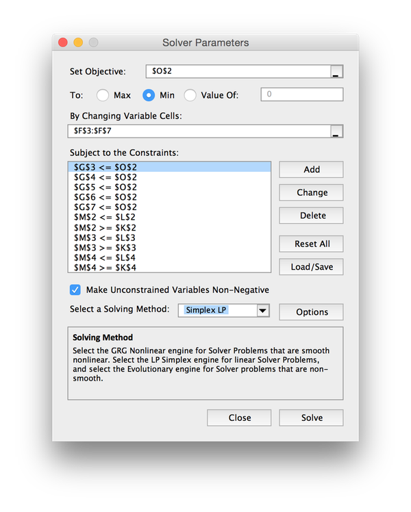
Enter the cell reference of the objective function in the topmost box.
Indicate whether the problem is a minimization or maximization problem using the radio buttons.
Enter the cell range of the decision variables in input box below that.
One enters the constaints one at a time by clicking the Add button, which brings up another dialog.
Note that there is a checkbox that can be used to indicate that all decision variables are non-negative.