INSTALL PYTHON
Mac
Install Homebrew. Install Python and a few command line tools:
$ brew install curl python python3
$ pip install virtualenv
Ubuntu
$ sudo apt install curl python2.7-dev python3-dev
$ sudo -H pip install virtualenv
INSTALL LIBRARIES
Install Python NLP libraries in a virtual environment:
$ virtualenv --python=python3 ve
$ . ve/bin/activate
$ pip3 install nltk numpy scipy scikit-learn gensim spaCy
$ python3 -m spacy.en.download
$ python3
>>> import nltk
>>> nltk.download_shell()
Use the NLTK downloader to install these packages:
- brown
- maxent_treebank_pos_tagger
- punkt
- reuters
- stopwords
- treebank
- wordnet
Download the complete Shakespeare in plain text:
$ curl http://www.gutenberg.org/cache/epub/100/pg100.txt \
  | gzcat \
  > /tmp/shakes.txt

$ wc /tmp/shakes.txt
  124787  904061 5589889 /tmp/shakes.txt
CHARACTER FREQUENCY
$ cat /tmp/shakes.txt \
| sed $'s/./&\\\n/g' \
| awk '{cnt[$0] += 1} END {for (i in cnt) print cnt[i], i}' \
| sort -nr
In the sed substitution, the & is a backreference to the string matched by the regular expression.
To put a newline in the sed script, use the $' ' style string available in bash and zsh.
An application of character frequency is breaking substitution ciphers. See http://norvig.com/mayzner.html for English letter frequency and a number of other properties of English text.
ASCII CHARACTER CLASSES
Unix tools and the C standard library define 12 or 13 standard character classes for partitioning the ASCII character set:
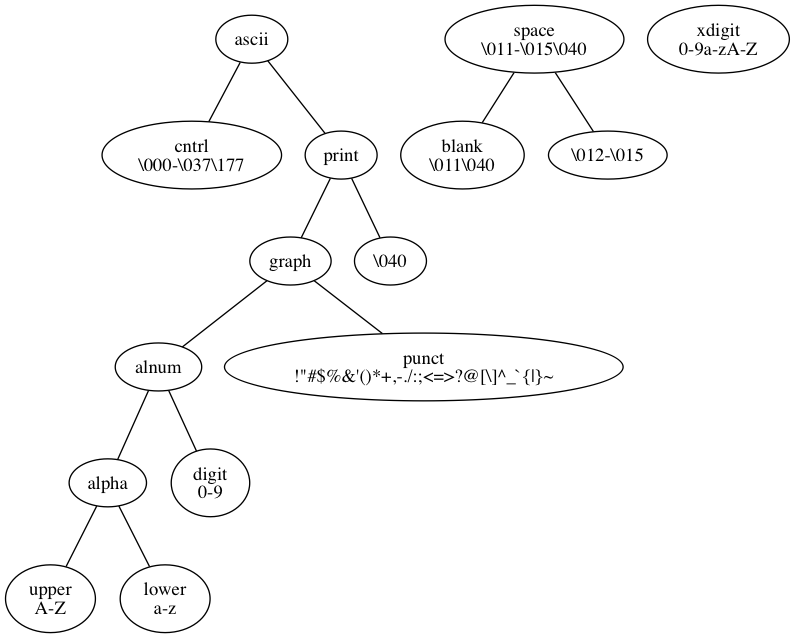
The character classes are used by the command line tool tr via the [:CLASS:] notation and in regular expressions via the [[:CLASS:]] notation.
A C character of type char or wchar_t can be tested using the isCLASS and iswCLASS functions which are defined in ctype.h and wctype.h.
| ascii | ||||||
|---|---|---|---|---|---|---|
| tr | tr | ctype.h | wctype.h | regex | regex | perl regex |
| '0-9a-zA-Z' | '[:alnum:]' | isalnum | iswalnum | [0-9a-zA-Z] | [[:alnum:]] | |
| '0-9a-zA-Z_' | [0-9a-zA-Z_] | \w | ||||
| 'a-zA-Z' | '[:alpha:]' | isalpha | iswalpha | [a-zA-Z] | []:alpha:]] | |
| '\000-\177' | isascii | iswascii | [\000-\177] | |||
| '\013\040' | '[:blank:]' | isblank | iswblank | [\013-\040] | ||
| '\000-\037\177' | '[:cntrl:]' | iscntrl | iswcntrl | [\000-\037\177] | [[:cntrl:]] | |
| '0-9' | '[:digit:]' | isdigit | iswdigit | [0-9] | [[:digit:]] | \d |
| '\041-\176' | '[:graph:]' | isgraph | isgraph | [\041-\176] | [[:graph:]] | |
| 'a-z' | '[:lower:]' | islower | iswlower | [a-z] | [[:lower:]] | |
| '\040-\176' | '[:print:]' | isprint | iswprint | [\040-\177] | [[:print:]] | |
| '!"#$%&'"'"'()*+,-./:;<=>?@[\]^_`{|}~' '\041-\057\072-\100\133-\140\173-\176' |
'[:punct:]' | ispunct | iswpunct | [[:punct:]] | ||
| ' \f\n\r\t\v' '\011-\015\040' |
'[:space:]' | isspace | iswspace | [\011-\015\040] | [[:space:]] | \s |
| 'A-Z' | '[:upper:]' | isupper | iswupper | [A-Z] | [[:upper:]] | |
| '0-9a-fA-F' | '[:xdigit:]' | isxdigit | iswxdigit | [0-9a-fA-F] | [[:xdigit:]] | |
POSIX specifies the list of characters in each of the character classes for a POSIX compliant system when the value of the LC_ALL environment variable is "POSIX" or "C". In these cases, the character classes only match ASCII characters and are as defined above.
If the LC_ALL environment variable is not defined, but the LC_CTYPE environment variable is, then it will be used to specify the list of characters in the character classes. If LC_CTYPE is not set, the LANG environment variable will be used.
CHARACTER N-GRAMS
#!/usr/bin/env python

import argparse
import codecs
import collections
import re
import sys
from operator import itemgetter

ENCODING = 'utf-8'

sys.stdin = codecs.getreader(ENCODING)(sys.stdin)
sys.stdout = codecs.getwriter(ENCODING)(sys.stdout)
sys.stderr = codecs.getwriter(ENCODING)(sys.stderr)

parser = argparse.ArgumentParser()
parser.add_argument('-n',
                    dest='n',
                    type=int,
                    required=True)
args = parser.parse_args()
count = collections.defaultdict(int)

clean_input = re.compile(r'[\t\n]').sub(' ', sys.stdin.read())

for idx in range(0, len(clean_input) - args.n):
    count[clean_input[idx:idx + args.n]] += 1

for ngram, cnt in reversed(sorted(count.iteritems(), key=itemgetter(1))):
    print(u'{}\t{}'.format(cnt, ''.join(ngram)))
One might not want n-grams which straddle word boundaries. This could be achieved with the above script by removing all characters except for letters and spaces. In the output, filter out the n-grams which contain a space.
EDIT DISTANCE
The Levenshtein distance is the minimum number of insertions, deletions, and substitutions of characters needed to convert one string into another.
Each insertion of a character or deletion of a character counts 1. Substituting a character for another also counts for 1.
$ python3
>>> import nltk
>>> from nltk.metrics.distance import edit_distance
>>> edit_distance("foo", "food")
1
>>> edit_distance("foo", "fop")
1
>>> edit_distance("foo", "ofo")
2
>>> edit_distance("foo", "ofo", True)
1
>>> edit_distance("foo", "oof", True)
2
Setting the 3rd argument to True computes the Damerau–Levenshtein distance, where transposition of adjacent characters also counts 1.
UNICODE PROPERTIES
Unicode characters are organized into categories and assigned properties:
Unicode general categories
Unicode character properties
Letters belong to a script:
As of Python 3, the character class abbreviations \d, \s, and \w will match non-ASCII characters. The re.A flag can be used to make them only match ASCII characters, which is the Python 2 behavior.
$ python3
>>> import re
>>> RX_WORD = re.compile(r'^\w+$')
>>> RX_WORD.search('λαμβδα')
<_sre.SRE_Match object; span=(0, 6), match='λαμβδα'>
>>> RX_ASCII_WORD = re.compile(r'^\w+$', re.A)
>>> RX_ASCII_WORD.search('λαμβδα')
TOKENIZE
$ python3
>>> import nltk
>>> nltk.tokenize.word_tokenize("Don't eat the yellow snow.")
['Do', "n't", 'eat', 'the', 'yellow', 'snow', '.']
$ python3
>>> import spacy
>>> nlp = spacy.en.English()
>>> doc = nlp("Don't eat the yellow snow.")
>>> print([str(tok) for tok in doc])
['Do', "n't ", 'eat ', 'the ', 'yellow ', 'snow', '.']
The graphical ASCII characters are the digits, letters, and punctuation:
    0-9
    A-Za-z
    !"#$%&'()*+,-./:;<=>?@[\]^_`{|}~
Here is a test to see how word_tokenize handles punctuation:
>>> for ch in "!\"#$%&'()*+,-./:;<=>?@[\\]^_`{|}~":
...   nltk.tokenize.word_tokenize(
...      ' ' + ch + 'foo' + ch + 'bar' + ch + ' ')
...
['!', 'foo', '!', 'bar', '!']
['``', 'foo', "''", 'bar', "''"]
['#', 'foo', '#', 'bar', '#']
['$', 'foo', '$', 'bar', '$']
['%', 'foo', '%', 'bar', '%']
['&', 'foo', '&', 'bar', '&']
["'foo'bar", "'"]
['(', 'foo', '(', 'bar', '(']
[')', 'foo', ')', 'bar', ')']
['*foo*bar*']
['+foo+bar+']
[',', 'foo', ',', 'bar', ',']
['-foo-bar-']
['.foo.bar', '.']
['/foo/bar/']
[':', 'foo', ':', 'bar', ':']
[';', 'foo', ';', 'bar', ';']
['<', 'foo', '<', 'bar', '<']
['=foo=bar=']
['>', 'foo', '>', 'bar', '>']
['?', 'foo', '?', 'bar', '?']
['@', 'foo', '@', 'bar', '@']
['[', 'foo', '[', 'bar', '[']
['\\foo\\bar\\']
[']', 'foo', ']', 'bar', ']']
['^foo^bar^']
['_foo_bar_']
['`foo`bar`']
['{', 'foo', '{', 'bar', '{']
['|foo|bar|']
['}', 'foo', '}', 'bar', '}']
['~foo~bar~']
This punctuation is treated as parts of words:
*+-/=\^_`|~
This punctuation is treated as standalone tokens:
!#$%&(),:;<>?@[]{}
This punctuation gets special treatment:
"'.
Double quotes are replaced with either two backquotes {{``}} or two single quotes {{'' depending upon whether they are the left or right double quotes.
The tokenizer also attempts to distinguish between single quotes used for quotation (separate token) and apostrophes (part of word). You may have noticed that don't parses as do and n't.
The tokenizer attempts to distinguish periods used for abbreviations (part of word) from sentence terminators (separate token).
Here is a command line tokenizer which discards the standalone punctuation tokens but otherwise approximates word_tokenize. Single quotes are preserved and double quotes are discarded:
tr -C '0-9a-zA-Z\047\052\053\055\057\075\134\136\137\140\174\176' ' '
WORD FREQUENCY
$ tr -c '0-9a-zA-Z\047\052\053\055\057\075\134\136\137\140\174\176' ' ' \
  < /tmp/shakes.txt \
  | tr -s ' ' | tr ' ' '\n' | sort | uniq -c | sort -nr
The Brown Corpus contains 500 samples of English text published in 1961:
$ python3 -c 'import nltk; print(" ".join(nltk.corpus.brown.words()))' \
  > /tmp/brown.txt

$ tr -c '0-9a-zA-Z\047\052\053\055\057\075\134\136\137\140\174\176' ' ' \
  < /tmp/brown.txt \
  | tr -s ' ' | tr ' ' '\n' | sort | uniq -c | sort -nr
BAG OF WORDS
scikit learn: Feature extraction
For many text processing algorithms, we ignore or discard the positions of words in a document and consider only the frequencies of the words. This is the bag of words representation of the document. Multiset is a synonym for bag in this context.
A simple way to represent a bag of words is as a list of strings. The count method can be used to get the word frequency:
>>> import nltk
>>> doc = "Sally sells sea shells by the sea shore."
>>> toks = nltk.tokenize.word_tokenize(doc)
>>> toks
['Sally', 'sells', 'sea', 'shells', 'by', 'the', 'sea', 'shore', '.']
>>> toks.count("sea")
2
Converting a list to a dict:
>>> import collections
>>> bow = collections.defaultdict(int)
>>> for toks in toks:
...     bow[tok] += 1
...
>>> bow
defaultdict(<type 'int'>, {'shells': 1, 'by': 1, 'shore': 1,
   'sea': 2, 'the': 1, '.': 1, 'Sally': 1, 'sells': 1})
>>> bow["sea"]
2
In the interest of performance, we might want to replace strings with integers. Here is how to do it with gensim:
>>> import gensim
>>> docs = ["Sally sells sea shells by the sea shore.",
...   "It was many and many a year ago,\nIn a kingdom by the sea,"]
>>> docs
['Sally sells sea shells by the sea shore.',
   'It was many and many a year ago,\nIn a kingdom by the sea,']
>>> bows = [nltk.tokenize.word_tokenize(doc) for doc in docs]
>>> dictionary = gensim.corpora.Dictionary(bows)
>>> corpus = [dictionary.doc2bow(bow) for bow in bows]
>>> corpus
[[(0, 1), (1, 1), (2, 1), (3, 1), (4, 2), (5, 1), (6, 1), (7, 1)],
   [(4, 1), (5, 1), (7, 1), (8, 1), (9, 2), (10, 1), (11, 2),
    (12, 1), (13, 1), (14, 2), (15, 1), (16, 1), (17, 1)]]
Use the id2token method to look up the token associated with an identifier:
>>> dictionary.id2token
{0: u'shells', 1: u'sells', 2: u'.', 3: u'shore', 4: u'sea', 5: u'the',
 6: u'Sally', 7: u'by', 8: u'and', 9: u'a', 10: u'ago', 11: u'many',
 12: u'year', 13: u'It', 14: u',', 15: u'In', 16: u'kingdom',
 17: u'was'}
>>> dictionary.id2token[4]
u'sea'
Replacing words with integers using scikit-learn:
>>> from sklearn.feature_extraction.text import CountVectorizer
>>> docs = ["Sally sells sea shells by the sea shore.",
...   "It was many and many a year ago,\nIn a kingdom by the sea,"]
>>> vectorizer = CountVectorizer()
>>> counts = vectorizer.fit_transform(docs)
>>> print(counts)
  (0, 7)	1
  (0, 9)	1
  (0, 8)	2
  (0, 10)	1
  (0, 2)	1
  (0, 12)	1
  (0, 11)	1
  (1, 8)	1
  (1, 2)	1
  (1, 12)	1
  (1, 4)	1
  (1, 13)	1
  (1, 6)	2
  (1, 1)	1
  (1, 14)	1
  (1, 0)	1
  (1, 3)	1
  (1, 5)	1
>>> vectorizer.vocabulary_
{u'and': 1, u'ago': 0, u'shells': 10, u'many': 6, u'year': 14,
   u'sally': 7, u'it': 4, u'sells': 9, u'shore': 11, u'sea': 8,
   u'in': 3, u'kingdom': 5, u'the': 12, u'was': 13, u'by': 2}
SPELL CHECK
$ echo 'foo bar is a bad worke' \
| tr ' ' '\n' \
| sort \
| comm -23 - /usr/share/dict/words
worke

$ brew install aspell
$ echo 'foo bar is a bad worke' | aspell list
worke
SENTENCE SEGMENTATION
Count the number of sentences in the Gettysburg Address:
$ curl http://clarkgrubb.wdfiles.com/local--files/nlp/getty.txt \
> /tmp/getty.txt

$ python3
>>> import nltk
>>> from nltk.tokenize import sent_tokenize
>>> with open('/tmp/getty.txt') as f:
...   s = f.read()
...
>>> len(sent_tokenize(s))
10
$ python3
>>> import spacy
>>> nlp = spacy.en.English()
>>> doc = nlp(open('/tmp/getty.txt').read())
>>> len(list(doc.sents))
11
STEMMING
Porter Stemming Algorithm Implementations
$ python3
>>> import nltk
>>> from nltk.stem.porter import PorterStemmer
>>> stemmer = PorterStemmer()
>>> stemmer.stem('walking')
'walk'
STOPWORDS
$ python3
>>> import nltk
>>> len(nltk.corpus.stopwords.words('english'))
127
Output the stopwords one per line:
$ python3 -c 'import nltk; '\
'print("\n".join(nltk.corpus.stopwords.words("english")))'
WORD N-GRAMS
Here is a source of natural language n-gram frequencies:
If we have our own corpus, we can calculate our own n-gram frequencies:
$ curl http://clarkgrubb.wdfiles.com/local--files/nlp/getty.txt \
> /tmp/getty.txt

$ python3
>>> from nltk.util import ngrams
>>> import nltk
>>> f = open('/tmp/getty.txt')
>>> tokens = nltk.tokenize.word_tokenize(f.read())
>>> fout = open('/tmp/ngrams.txt', 'w')
>>> bigrams = ngrams(tokens, 2)
>>> for p in bigrams:
...  fout.write('|'.join(p) + '\n')
...
>>> fout.close()
The scikit learn CountVectorizer can also be used to extract n-grams:
>>> from sklearn.feature_extraction.text import CountVectorizer
>>> getty = open('/tmp/getty.txt').read()
>>> vectorizer = CountVectorizer(ngram_range=(2,2))
>>> analyzer = vectorizer.build_analyzer()
>>> bigrams = analyzer(getty)
>>> bigrams[0:10]
['fourscore and', 'and seven', 'seven years', 'years ago',
 'ago our', 'our fathers', 'fathers brought', 'brought forth',
 'forth on', 'on this']
If the n-grams are being used for creating features:
>>> from sklearn.feature_extraction.text import CountVectorizer
>>> getty = open('/tmp/getty.txt').read()
>>> vectorizer = CountVectorizer(ngram_range=(2,2))
>>> X = vectorizer.fit_transform([getty])
The return value of CountVectorizer.fit_transform is a matrix of integers representing the number of occurrences of the column (the n-gram id) in the row (the document).
CountVectorizer.vocabulary_ with a trailing underscore is a dictionary which maps the n-grams to their integer values. CountVectorizer.get_feature_names() will return an array with the n-grams in the order of their identifiers. Thus one can recover the n-gram strings with:
>>> pairs = list(zip(vectorizer.get_feature_names(), X.toarray()[0]))
>>> pairs[0:10]
[('above our', 1), ('add or', 1), ('advanced it', 1), ('ago our', 1),
 ('all men', 1), ('altogether fitting', 1), ('and dead', 1),
 ('and dedicated', 1), ('and proper', 1), ('and seven', 1)]
Some of the named parameters available when invoking the CountVectorizer constructor:
| param | values | description |
|---|---|---|
| analyzer | 'word', 'char', 'char_wb' | Use 'char' for character n-grams; 'char_wb' for character n-grams within words |
| binary | False, True | if True, value is 0 or 1 |
| lowercase | True, False | |
| max_df | 1.0 | float are percentage; integer for count |
| min_df | 1 | float for percentage; integer for count |
| ngram_range | (1, 1) | |
| stopwords | None, 'english' | or can be list of strings |
| strip_accents | None, 'ascii', 'unicode' | |
| token_pattern | '(?u)\\b\\w\\w+\\b' | a regular expression; (?u) is same as re.U and changes \w, \W, \b, \B, \d, \D, \s, \S |
TF-IDF
The term frequency is the number of times a term occurs in a document. If t is the term and d is the document, then this is written
(1)The inverse document frequency is defined for a term t and a corpus of documents D as:
(2)The tf-idf of the triple t, d, and D is
(3)
$ python3
>>> from sklearn.feature_extraction.text import TfidfVectorizer
>>> docs = [
...   'In Xanadu did Kubla Khan',
...   'A stately pleasure-dome decree:',
...   'Where Alph, the sacred river, ran',
...   'Through caverns measureless to man',
...   'Down to a sunless sea.',
...   'So twice five miles of fertile ground',
...   'With walls and towers were girdled round;',
...   'And there were gardens bright with sinuous rills,',
...   'Where blossomed many an incense-bearing tree;',
...   'And here were forests ancient as the hills,',
...   'Enfolding sunny spots of greenery.']
...
>>> vectorizer = TfidfVectorizer()
>>> data = vectorizer.fit_transform(docs)
>>> data.toarray()
WORDNET
Morphological form to a lemma:
$ python3
>>> import nltk
>>> from nltk.stem.wordnet import WordNetLemmatizer
>>> wnl = WordNetLemmatizer()
>>> wnl.lemmatize('dogs')
'dog'
Senses of a word:
>>> from nltk.corpus import wordnet
>>> wordnet.synsets('dog')
[Synset('dog.n.01'), Synset('frump.n.01'), Synset('dog.n.03'),
 Synset('cad.n.01'), Synset('frank.n.02'), Synset('pawl.n.01'),
 Synset('andiron.n.01'), Synset('chase.v.01')]
Definition and lemmas for a sense:
>>> dog = wordnet.synset('dog.n.01')
>>> dog.definition()
'''a member of the genus Canis (probably descended from the
 common wolf) that has been domesticated by man since
 prehistoric times; occurs in many breeds'''
>>> dog.lemmas()
[Lemma('dog.n.01.dog'), Lemma('dog.n.01.domestic_dog'),
 Lemma('dog.n.01.Canis_familiaris')]
Hypernyms and hyponyms (i.e. superclasses and subclasses):
>>> dog = wordnet.synset('dog.n.01')
>>> dog.hypernyms()
[Synset('canine.n.02'), Synset('domestic_animal.n.01')]
>>> len(dog.hyponyms())
18
Meronyms (i.e. parts of the whole):
>>> car = wordnet.synset('car.n.01')
>>> car.part_meronyms()
[Synset('accelerator.n.01'), Synset('air_bag.n.01'),
Synset('auto_accessory.n.01'), Synset('automobile_engine.n.01'),
Synset('automobile_horn.n.01'), Synset('buffer.n.06'),
Synset('bumper.n.02'), Synset('car_door.n.01'),
Synset('car_mirror.n.01'), Synset('car_seat.n.01'),
Synset('car_window.n.01'), Synset('fender.n.01'),
Synset('first_gear.n.01'), Synset('floorboard.n.02'),
Synset('gasoline_engine.n.01'), Synset('glove_compartment.n.01'),
Synset('grille.n.02'), Synset('high_gear.n.01'), Synset('hood.n.09'),
Synset('luggage_compartment.n.01'), Synset('rear_window.n.01'),
Synset('reverse.n.02'), Synset('roof.n.02'),
Synset('running_board.n.01'), Synset('stabilizer_bar.n.01'),
Synset('sunroof.n.01'), Synset('tail_fin.n.02'),
Synset('third_gear.n.01'), Synset('window.n.02')]
PART OF SPEECH
Brown Corpus POS Tags (87)
Penn Treebank POS Tags (45)
The BNC Basic (C5) Tagset (61)
$ python3
>>> import nltk
>>> s = "Don't eat the yellow snow."
>>> nltk.pos_tag(nltk.tokenize.word_tokenize(s))
[('Do', 'NNP'), ("n't", 'RB'), ('eat', 'VB'), ('the', 'DT'),
 ('yellow', 'JJ'), ('snow', 'NN'), ('.', '.')]
The NLTK POS tagger mis-classifies the first token, but the spaCy tagger does better:
$ python3
>>> import spacy
>>> nlp = spacy.en.English()
>>> doc = nlp("Don't eat the yellow snow.")
>>> [nlp.vocab.strings[doc[i].tag] for i in range(0, len(list(doc)))]
['VB', 'RB', 'VB', 'DT', 'JJ', 'NN', '.']
PARSER
The Stanford Parser:
$ curl http://nlp.stanford.edu/software/stanford-parser-full-2015-01-29.zip > stanford-parser-full-2015-01-29.zip
$ unzip stanford-parser-full-2015-01-29.zip
$ cd stanford-parse-full-2015-01-30
$ echo $'How many birds are sitting in the tree?' > /tmp/test.txt
$ ./lexparser.sh /tmp/test.txt 2> /dev/null
(ROOT
  (SBARQ
    (WHNP
      (WHADJP (WRB How) (JJ many))
      (NNS birds))
    (SQ
      (VP (VBP are)
        (VP (VBG sitting)
          (PP (IN in)
            (NP (DT the) (NN tree))))))
    (. ?)))

advmod(many-2, How-1)
amod(birds-3, many-2)
nsubj(sitting-5, birds-3)
aux(sitting-5, are-4)
root(ROOT-0, sitting-5)
det(tree-8, the-7)
prep_in(sitting-5, tree-8)

(ROOT
  (S
    (VP (VB Make)
      (NP (PRP it))
      (ADVP (RB so)))
    (. !)))

root(ROOT-0, Make-1)
dobj(Make-1, it-2)
advmod(Make-1, so-3)
spaCy:
$ cat tree.py
def get_root(doc):
    tok = doc[0]
    while tok != tok.head:
        tok = tok.head

    return tok


def print_node(nlp, node, indent):
    print((' ' * indent) + nlp.vocab.strings[node.tag] + ' ' + str(node))
    for tok in node.children:
        if tok != node:
            print_node(nlp, tok, indent + 2)


def print_doc(nlp, doc):
    root = get_root(doc)
    print_node(nlp, root, indent=0)

$ python3
>>> import spacy
>>> nlp = spacy.en.English()
>>> doc = nlp('How many birds are sitting in the tree?\nMake it so!')
>>> import tree
>>> tree.print_doc(nlp, doc)
VBG sitting
  NNS birds
    JJ many
      WRB How
  VBP are
  IN in
    NN tree
      DT the
  . ?
NAIVE BAYES
Let Ck be the chance that a document with features x1 ... ,xn belongs to class k. Then according to Bayes rule and the chain rule for conditional probability:
(4)If we make the naive assumption that the features are independent, we get a simpler formula:
(5)If we have a representative sample of data, we can use it to estimate the P(Ck) and the P(xi|Ck). If we are only interested in the mostly likely class for a document, we don't bother to compute the P(xi) since they are the same for all classes. We classify a document by choosing the class for which
(6)is highest.
>>> import nltk
>>> def features(s):
...     vec = {}
...     for token in nltk.tokenize.word_tokenize(s):
...         vec[token] = 1 if token not in vec else vec[token] + 1
...
...     return vec
...
>>> data = [('Hi John, I will see you at 9:00pm', 'ham'),
...         ('Buy Viagra at low, low prices.  One time offer.', 'spam'),
...         ('Your Amazon Order is for the book "Harry Potter"', 'ham'),
...         ('Earn a million dollars by working at home.', 'spam')]
...
>>> processed_data = [(features(tup[0]), tup[1]) for tup in data]
>>> classifier = nltk.NaiveBayesClassifier.train(processed_data)
>>> classifier.classify(features("This is good Viagra!"))
'spam'
>>> classifier.classify(features("We will meet you at 7pm.  Take care"))
'ham'
TOPIC MODEL: LSA
When we represent a set of documents by indexed features, we can put our data in the form of a matrix in which the rows represent documents and the columns represent features. In the case of bag-of-words features, the matrix is sparse, meaning most of the entries are zero. The number of features is the number of words in the data set, and is often in the thousands.
Latent semantic analysis (LSA) is a technique for finding a "nearby" matrix with fewer features. We can specify the number of features we want. The technique involves performing a singular value decomposition on the original matrix. The dimensions of the new matrix will be smaller, but it will also be dense, so it might not consume less memory.
Let's get a set of documents. They are Reuters news articles drawn from four different categories:
$ python3
>>> from nltk.corpus import reuters
>>> CATEGORIES = ['coffee', 'housing', 'money-supply', 'rubber']
>>> data = []
>>> for cat in CATEGORIES:
...    data.extend([{'label': cat, 'document': reuters.raw(fid)}
...       for fid
...       in reuters.fileids(cat)])
...
>>> len(data)
382
>>> import collections
>>> cat_to_cnt = collections.defaultdict(int)
>>> for row in data:
...   cat_to_cnt[row['label']] += 1
...
>>> cat_to_cnt
defaultdict(<class 'int'>, {'housing': 20, 'coffee': 139,
    'money-supply': 174, 'rubber': 49})
Next create the features. We use TF-IDF to de-emphasize the importance of common words:
>>> docs = [d['document'] for d in data]
>>> from sklearn.feature_extraction.text import TfidfVectorizer
>>> vectorizer = TfidfVectorizer()
>>> tfidfs = vectorizer.fit_transform(docs)
Perform the SVD decomposition:
>>> import numpy
>>> tfidfs.toarray().shape
(382, 5492)
>>> u, s, v = numpy.linalg.svd(tfidfs.toarray())
The singular values in s are in decreasing order. We want the biggest values. It is worthwhile to consider the fraction of "information" that we are preserving when we discard singular values:
>>> sum(s[:100]) / sum(s)
0.60941954345568206
>>> sum(s[:200]) / sum(s)
0.81150074754767521
>>> sum(s[:300]) / sum(s)
0.95132368373281095
We take the top 100 singular values:
>>> lsa = numpy.dot(u, numpy.diag(s)[:,:100])
>>> lsa.shape
(382, 100)
Next we see how well a clustering technique distinguishes the original clusters:
>>> from sklearn.cluster import KMeans
>>> kmeans = KMeans(n_clusters=4, random_state=0).fit(lsa)
>>> kmeans.labels_
array(
 [1, 1, 3, 0, 0, 3, 1, 1, 3, 1, 2, 0, 1, 0, 2, 0, 1, 0, 1, 0, 0, 3, 0,
  0, 3, 3, 1, 0, 1, 1, 1, 1, 3, 1, 1, 1, 1, 2, 1, 1, 1, 0, 1, 1, 1, 2,
  0, 0, 2, 1, 1, 1, 0, 3, 3, 3, 0, 1, 1, 2, 0, 1, 3, 0, 1, 2, 1, 0, 0,
  3, 2, 2, 3, 0, 2, 3, 3, 2, 0, 1, 1, 3, 0, 3, 1, 0, 3, 3, 1, 0, 3, 0,
  1, 1, 0, 1, 1, 3, 0, 3, 1, 1, 1, 1, 0, 1, 2, 1, 2, 1, 0, 1, 0, 2, 0,
  0, 0, 1, 1, 1, 2, 1, 3, 3, 2, 3, 0, 2, 3, 0, 1, 0, 1, 2, 1, 3, 0, 2,
  1, 2, 3, 3, 1, 1, 1, 1, 1, 1, 1, 3, 3, 3, 3, 2, 2, 3, 3, 2, 3, 0, 2,
  0, 2, 0, 3, 2, 3, 2, 1, 3, 1, 2, 2, 2, 1, 3, 1, 3, 3, 3, 3, 0, 1, 2,
  2, 1, 2, 2, 3, 1, 3, 1, 1, 1, 2, 1, 3, 2, 3, 2, 2, 2, 2, 1, 2, 1, 2,
  2, 1, 3, 0, 2, 2, 1, 3, 2, 1, 0, 2, 1, 3, 3, 2, 1, 3, 1, 3, 3, 1, 1,
  2, 0, 1, 0, 3, 3, 0, 3, 3, 2, 1, 1, 2, 3, 2, 3, 3, 2, 3, 3, 1, 2, 2,
  2, 1, 1, 0, 1, 3, 1, 3, 3, 2, 3, 2, 3, 2, 2, 1, 2, 3, 2, 3, 2, 2, 2,
  2, 2, 2, 2, 2, 2, 3, 1, 2, 1, 3, 3, 1, 2, 3, 3, 3, 2, 3, 3, 1, 1, 3,
  2, 3, 2, 3, 1, 2, 1, 2, 2, 0, 2, 2, 3, 1, 1, 2, 2, 2, 2, 2, 0, 1, 1,
  1, 1, 3, 0, 3, 2, 2, 2, 3, 1, 1, 0, 1, 2, 1, 2, 0, 1, 2, 2, 0, 3, 3,
  0, 3, 0, 1, 3, 3, 1, 2, 1, 1, 3, 1, 1, 0, 3, 3, 3, 2, 3, 1, 3, 1, 2,
  1, 2, 3, 1, 2, 3, 0, 2, 0, 3, 0, 1, 1, 3], dtype=int32)
>>> cnt = {}
>>> for label in CATEGORIES:
...    cnt[label] = [0, 0, 0, 0]
>>> for i in range(0, 382):
...   cnt[data[i]['label']][kmeans.labels_[i]] += 1
>>> cnt
{'housing': [0, 7, 4, 9], 'coffee': [38, 55, 19, 27],
 'money-supply': [13, 45, 66, 50], 'rubber': [9, 15, 10, 15]}
Not much better than random. If we use 300 features instead of 100 the results are noticeably better:
>>> cnt
{'housing': [14, 5, 0, 1], 'coffee': [55, 59, 18, 7],
 'money-supply': [113, 41, 9, 11], 'rubber': [16, 24, 9, 0]}
TOPIC MODEL: LDA
SENTIMENT ANALYSIS
movie review data
Christopher Potts Tokenizer
Brendan O'Connor Tokenizer
The simplest sentiment analysis task is to say whether a text has a positive or negative attitude towards some entity. In some situations, such as movie reviews, it might be easy to identify the entity, but in other situations, such as tweets, the entity must be extracted from the text.
Scherer's Typology.
Tokenization issues: might want to preserve case, since all caps is like shouting. Punctuation used for emoticons is important. Normalize dates and phone numbers?
Negation: Sanjiv Das and Mike Chen technique: add NOT_ to every word after a negating word up to the next punctuation. This doubles the size of the vocabulary.
NAMED ENTITY RECOGNITION
Download the Stanford NER zip archive from http://nlp.stanford.edu/software/CRF-NER.shtml
$ unzip stanford-ner-2015-12-09.zip
$ cd stanford-ner-2015-12-09

$ cat sample.txt
The fate of Lehman Brothers, the beleaguered investment bank, hung in
the balance on Sunday as Federal Reserve officials and the leaders of
major financial institutions continued to gather in emergency meetings
trying to complete a plan to rescue the stricken bank.  Several
possible plans emerged from the talks, held at the Federal Reserve
Bank of New York and led by Timothy R. Geithner, the president of the
New York Fed, and Treasury Secretary Henry M. Paulson Jr.

$ java -mx600m -cp 'stanford-ner.jar:lib/*' \
    edu.stanford.nlp.ie.crf.CRFClassifier \
    -loadClassifier classifiers/english.all.3class.distsim.crf.ser.gz \
    -textFile sample.txt
The/O fate/O of/O Lehman/ORGANIZATION Brothers/ORGANIZATION
,/O the/O beleaguered/O investment/O bank/O ,/O hung/O in/O the/O
balance/O on/O Sunday/O as/O Federal/ORGANIZATION
Reserve/ORGANIZATION officials/O and/O the/O leaders/O of/O major/O
financial/O institutions/O continued/O to/O gather/O in/O emergency/O
meetings/O trying/O to/O complete/O a/O plan/O to/O rescue/O the/O
stricken/O bank/O ./O Several/O possible/O plans/O emerged/O from/O
the/O talks/O ,/O held/O at/O the/O Federal/ORGANIZATION
Reserve/ORGANIZATION Bank/ORGANIZATION of/ORGANIZATION
New/ORGANIZATION York/ORGANIZATION and/O led/O by/O
Timothy/PERSON R./PERSON Geithner/PERSON ,/O the/O president/O
of/O the/O New/ORGANIZATION York/ORGANIZATION Fed/ORGANIZATION
,/O and/O Treasury/ORGANIZATION Secretary/O Henry/PERSON
M./PERSON Paulson/PERSON Jr./PERSON ./O
>>> import spacy
>>> nlp = spacy.en.English()
>>> doc = nlp(open('sample.txt').read())
>>> doc.ents
(Lehman Brothers, Sunday, Federal Reserve, the Federal Reserve Bank,
New York, Timothy R. Geithner, the New York Fed, Treasury,
Henry M. Paulson Jr.)
RELATION EXTRACTION
The OpenIE license prohibits commerical use.
$ git clone https://github.com/knowitall/openie
$ cd openie
$ sbt package
$ sbt 'run-main edu.knowitall.openie.OpenIECli’
> WhatsApp 2.12.9 brings 3D Touch gestures to iPhone 6s: Download now http://t.co/YI7m2vutlR http://t.co/qubfpGuWmo
0.95 (WhatsApp 2.12.9; brings; 3D Touch gestures; to iPhone 6s)
> How Will Record iPhone 6s, 6s Plus Sales Affect Apple, AAPL, Earnings? http://t.co/E8RfDMblmG #Bing
0.94 (Will Record iPhone 6s; Affect; Apple, AAPL, Earnings)
Running OpenIE in batch mode:
$ echo 'WhatsApp 2.12.9 brings 3D Touch gestures to iPhone 6s: Download now http://t.co/YI7m2vutlR http://t.co/qubfpGuWmo' > /tmp/input.txt

$ echo 'How Will Record iPhone 6s, 6s Plus Sales Affect Apple, AAPL, Earnings? http://t.co/E8RfDMblmG #Bing' >> /tmp/input.txt

$ sbt -J-Xmx2700M clean compile assembly

$ java -Xmx4g -XX:+UseConcMarkSweepGC \
    -jar ./target/scala-2.10/openie-assembly-4.1.4-SNAPSHOT.jar \
    --format column \
    < /tmp/input.txt
JAPANESE: READING, DICTIONARY FORM, PART-OF-SPEECH
Mac:
$ brew install juman
Ubuntu:
$ sudo apt-get install juman
You can also download the tarball from http://nlp.ist.i.kyoto-u.ac.jp/EN/index.php?JUMAN and build from source.
$ echo ちょっと日本語分かりますけど。 | juman -b
ちょっと ちょっと ちょっと 副詞 8 * 0 * 0 * 0 "代表表記:ちょっと/ちょっと 相対名詞修飾 用言弱修飾"
日本 にほん 日本 名詞 6 地名 4 * 0 * 0 "代表表記:日本/にほん 地名:国"
語 ご 語 名詞 6 普通名詞 1 * 0 * 0 "代表表記:語/ご 漢字読み:音 カテゴリ:抽象物"
分かり わかり 分かる 動詞 2 * 0 子音動詞ラ行 10 基本連用形 8 "代表表記:分かる/わかる"
ます ます ます 接尾辞 14 動詞性接尾辞 7 動詞性接尾辞ます型 31 基本形 2 "代表表記:ます/ます"
けど けど けど 助詞 9 接続助詞 3 * 0 * 0 NIL
。 。 。 特殊 1 句点 1 * 0 * 0 NIL
EOS

$ echo アルバイトの若い人でしたよ。| juman -b
アルバイト あるばいと アルバイト 名詞 6 サ変名詞 2 * 0 * 0 "代表表記:アルバイト/あるばいと カテゴリ:人;抽象物 ドメイン:ビジネス"
の の の 助詞 9 格助詞 1 * 0 * 0 NIL
若い わかい 若い 形容詞 3 * 0 イ形容詞アウオ段 18 基本形 2 "代表表記:若い/わかい"
人 じん 人 名詞 6 普通名詞 1 * 0 * 0 "代表表記:人/じん 漢字読み:音 カテゴリ:人"
でした でした だ 判定詞 4 * 0 判定詞 25 デス列タ形 30 NIL
よ よ よ 助詞 9 終助詞 4 * 0 * 0 NIL
。 。 。 特殊 1 句点 1 * 0 * 0 NIL
EOS

$ echo 東京へ行った。 | juman -b
東京 とうきょう 東京 名詞 6 地名 4 * 0 * 0 "代表表記:東京/とうきょう 地名:日本:都"
へ へ へ 助詞 9 格助詞 1 * 0 * 0 NIL
行った いった 行く 動詞 2 * 0 子音動詞カ行促音便形 3 タ形 10 "代表表記:行く/いく 付属動詞候補(タ系) ドメイン:交通 反義:動詞:帰る/かえる"
。 。 。 特殊 1 句点 1 * 0 * 0 NIL
EOS

$ echo 鈴木さんは優しい人ですね。 | juman -b
鈴木 すずき 鈴木 名詞 6 人名 5 * 0 * 0 "人名:日本:姓:1:0.00961"
さん さん さん 接尾辞 14 名詞性名詞接尾辞 2 * 0 * 0 "代表表記:さん/さん"
は は は 助詞 9 副助詞 2 * 0 * 0 NIL
優しい やさしい 優しい 形容詞 3 * 0 イ形容詞イ段 19 基本形 2 "代表表記:優しい/やさしい"
人 じん 人 名詞 6 普通名詞 1 * 0 * 0 "代表表記:人/じん 漢字読み:音 カテゴリ:人"
です です だ 判定詞 4 * 0 判定詞 25 デス列基本形 27 NIL
ね ね ね 助詞 9 終助詞 4 * 0 * 0 NIL
。 。 。 特殊 1 句点 1 * 0 * 0 NIL
EOS
juman reads from standard input and writes out a single line for each word part or punctuation that it identifies. There is a separate line for each noun in a compound noun: e.g. 日本語 "Japanese language" gets two lines. Also 分かります "understands" gets two lines, one for the verb root and one for the suffix.
The first column in the output contains the characters in the input that were identified as belonging to the word part or punctuation.
The second column is the reading of the first column in hiragana. If the first column was already in hiragana then it is the same as the first column. Kanji characters have multiple readings and choosing the correct reading is difficult to do programmatically.
The third column is the dictionary form of the word, useful if you want to look the word up in a dictionary.
The fourth column is the part of speech.
| ja | en |
|---|---|
| 名詞 | noun |
| 動詞 | verb |
| 形容詞 | adjective |
| 副詞 | adverb |
| 助動詞 | auxiliary verb |
| 判定詞 | determiner |
| 助詞 | particle |
| 終助詞 | final particle |
| 格助詞 | case particle |
| 接尾辞 | suffix |
| 特殊 | special (used for punctuation) |
The sixth column gives more information about proper nouns. For 東京 "Tokyo" the 6th column is 地名 "place name" and for 鈴木 "Suzuki" it is 人名 "a person's name".
There are twelve columns, separated by spaces. The 12th column is sometimes double quoted and itself may contain spaces. I wasn't able to find information on the meaning of the other columns.
CHINESE: WORD SEGMENTATION
The Stanford NLP Group provides a Java app which can identify the words in Chinese text. The tool expects an input file with one sentence per line.
$ curl https://nlp.stanford.edu/software/stanford-segmenter-2018-02-27.zip > stanford-segmenter-2018-02-27.zip
$ tar xf stanford-segmenter-2018-02-27.zip
$ cd stanford-segmenter-2018-02-27

$ cat chinese.txt
霍洛威的双亲批评阿鲁巴警方在案件调查及质询最后看到他们女儿的三名男子期间工作有欠严谨,还呼吁杯葛阿鲁巴并得到亚拉巴马州州长鲍勃·赖利支持,但没有获得联邦层面的支持。
2012年1月12日,亚拉巴马州法官宣告娜塔莉·安·霍洛威在法律上已经死亡。

$ ./segment.sh ctb chinese.txt UTF-8 0
霍洛威 的 双亲 批评 阿鲁巴 警方 在 案件 调查 及 质询 最后 看到 他们 女儿 的 三 名 男子 期间 工作 有欠 严谨 , 还 呼吁 杯葛 阿鲁巴 并 得到 亚拉巴马州 州长 鲍勃·赖利 支持 , 但 没有 获得 联邦 层面 的 支持 。
2012年 1月 12日 , 亚拉巴马州 法官 宣告 娜塔莉·安·霍洛威 在 法律 上 已经 死亡 。