a tour of statistical learning using R and scikit-learn
intro | r | scikit learn
nearest neighbors | linear regression | logistic regression | linear discriminant analysis | naive bayes | support vector machine | decision tree | random forest | boosting | neural network
intro
Statistical learning is a set of techniques for building a model which attempts to predict a response variable from one or more predictor variables.
Labeled data are tuples of predictor values with their associated response values. Typically one divides the labeled data into a training set and a test set. The model is built using the training set and then the test set is used to evaluate the performance of the model.
The test set guards against overfitting, which is when a model performs well on the data used to train it, but poorly on unseen data.
Variables can be quantitative or categorical. When a variable is categorical, it can take one of k of unordered values. We can convert a categorical variable to k-1 dummy variables. At most one of the dummy variables can be set to 1 and all of the categorical variables are 0 when the categorical variable has the baseline value.
When the response variable is quantitative, a model which predicts it is said to be a regression model. When the response variable is categorical, the model is a classification model.
r
How to list the variables in scope and how to inspect their type:
> x = 3
> ls()
[1] "x"

> class(x)
[1] "numeric"
> str(x)
 num 3
How to get documentation for a function:
> ?mean
R has a data type called data frame which equivalent to a relational database table.
The variable iris is always in scope and contains a data frame:
> dim(iris)
[1] 150   5

> names(iris)
[1] "Sepal.Length" "Sepal.Width"  "Petal.Length" "Petal.Width"  "Species"
The columns are vectors and can be accessed using index notation, dollar sign notation, or the with command. Notice the difference in type of the last expression:
> class(iris[, "Sepal.Length"])
[1] "numeric"

> class(iris$Sepal.Length)
[1] "numeric"

> with(iris, class(Sepal.Length))
[1] "numeric"

> class(iris["Sepal.Length"])
[1] "data.frame"
The attach command makes all of the columns available as variables:
> attach(iris)
> class(Sepal.Length)
[1] "numeric"
How to get a single row of a data frame:
> iris[1, ]
  Sepal.Length Sepal.Width Petal.Length Petal.Width Species
1          5.1         3.5          1.4         0.2  setosa

> class(iris[1, ])
[1] "data.frame"
The columns of a data frame can have different types:
> class(iris$Species)
[1] "factor"
explain factors
loading data
scikit learn
scikit-learn is a Python library which can be installed with pip:
$ sudo pip install scikit-learn
scikit-learn uses numpy, which is a Python library which provides a homogeneous multidimensional type called ndarray.
>>> from sklearn.datasets import load_iris
>>> iris = load_iris()

>>> type(iris.data)
<class 'numpy.ndarray'>

>>> iris.data.ndim
2
>>> iris.data.shape
(150, 4)

>>> iris.data[0, 0]
5.0999999999999996
>>> iris.data[0, :]
array([ 5.1,  3.5,  1.4,  0.2])
>>> iris.data[0:3, :]
array([[ 5.1,  3.5,  1.4,  0.2],
       [ 4.9,  3. ,  1.4,  0.2],
       [ 4.7,  3.2,  1.3,  0.2]])
scipy sparse arrays
load_svmlight_file
nearest neighbors
The idea is to find the k nearest neighbors in the labeled data to an unlabeled tuple and use them to make the prediction. If the response is numeric, average the neighbors. If the response is categorical, use majority rule.
> require('class')

> nrow(iris)
[1] 150
> names(iris)
[1] "Sepal.Length" "Sepal.Width"  "Petal.Length" "Petal.Width"  "Species"
> train = sample(1:nrow(iris), 100)
> iris.predictors = iris[, c("Sepal.Length", "Sepal.Width", "Petal.Length", "Petal.Width")]
> iris.response = iris[, c("Species")]
> train = runif(150) > 0.5
> knn.model = knn(iris.predictors[train, ], iris.predictors[!train, ], iris.response[train], k=3)
> table(knn.model, iris.response[!train])

knn.model    setosa versicolor virginica
  setosa         21          0         0
  versicolor      0         26         0
  virginica       0          4        21
> mean(knn.model == iris.response[!train])
[1] 0.9444444
Nearest neighbors works best when there is lots of input data and four or fewer predictors.
The reason that lots of predictors don't work well is because in high dimensions, the k nearest neighbors are often quite far away.
Here is a graph showing the radius of the p-sphere needed to include a given fraction of the predictors, assuming that they are uniformly distributed in the unit p-cube. The dotted line marks the radius of the p-spheres which include 10% of the predictors.
> x = seq(0, 1, .01)
> plot(x, x, type='l', xlab='fraction volume of unit n-cube', ylab='radius of sphere')
> lines(x, x^.5, col='red')
> lines(x, x^.33333333, col='green')
> lines(x, x^.25, col='orange')
> lines(x, x^.1, col='blue')
> lines(x, x^.2, col='purple')
> lines(rep(.1, 101), seq(0, 1, .01), lty=3, col='gray')
> lines(rep(.1, 101), seq(0, 1, .01), lty=3)
> legend('bottomright', c('p=1', 'p=2', 'p=3', 'p=4', 'p=5', 'p=10'), lty=c(1,1,1,1,1,1), lwd=c(2.5,2.5,2.5,2.5,2.5,2.5), col=c('black', 'red', 'green', 'orange', 'purple', 'blue'))
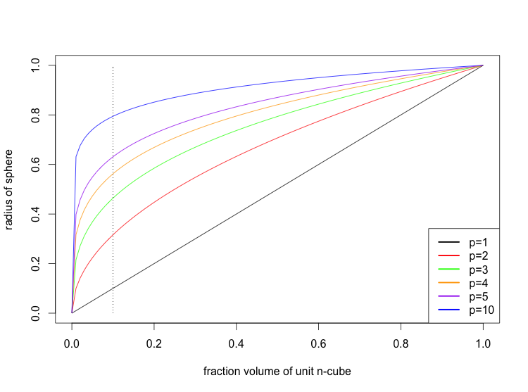
The situation is actually somewhat worse than depicted because in high dimensions the p-sphere must often extend outside of the p-cube.
scikit-learn:
>>> from sklearn.datasets import load_iris
>>> from sklearn.neighbors import KNeighborsClassifier
>>> iris = load_iris()

>>> train = sample(range(0, 150), 75)
>>> test = [i for i in range(0, 150) if i not in train]

>>> clf = KNeighborsClassifier(n_neighbors=5)
>>> clf = clf.fit(iris.data[train], iris.target[train])

>>> confusion_matrix(clf.predict(iris.data[test]), iris.target[test])
array([[22,  0,  0],
       [ 0, 24,  1],
       [ 0,  1, 27]])
>>> sum([1 if x else 0 for x in clf.predict(iris.data[test]) == iris.target[test]]) / len(test)
0.9733333333333334
Nearest neighbors has a parameter k which must be chosen. One way to choose it is to plot the test error for values of k:
> require('class')

> train = sample(1:nrow(iris), 100)
> iris.predictors = iris[, c("Sepal.Length", "Sepal.Width", "Petal.Length", "Petal.Width")]
> iris.response = iris[, c("Species")]
> train = runif(150) > 0.5

> test.err = rep(0, 15)

> for (i in 1:15) {
+   knn.model = knn(iris.predictors[train, ], iris.predictors[!train, ], iris.response[train], k=i)
+   test.err[i] = 1 - mean(knn.model == iris.response[!train])
+ }

> plot(1:15, test.err, xlab='k')
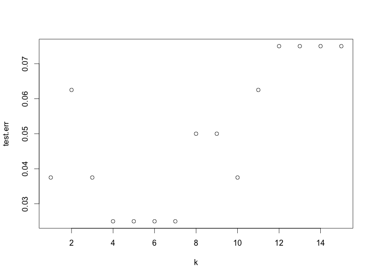
The plot shows 4 ≤ k ≤ 7 works best.
We note that if the test data is used to choose a parameter, then it cannot be used to estimate the accuracy of the final model. Hence, when training a model with a tunable parameter, we may split the data into three sets: training, validation, and test. The validation set is used to choose the parameter.
There a few ways to implement nearest neighbors. The brute force method checks every point in the training set to find the nearest neighbors. One must keep a list of the k nearest neighbors found so far. This is a O(nk) algorithm, or O(n log k) if a priority queue is used for the list of k nearest neighbors.
K-d trees and ball trees are data structures which can be used to index the location of the points in the training set. Whether they improve performance depends on the data; they are generally ineffective in high dimensions.
linear regression
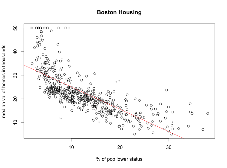
Linear regressions builds a model which is linear in the predictor variables. Usually the data overdetermines the model. The customary way to deal with this is to select the model which minimizes the sum of the squares of the residuals, which are the differences between the predicted and actual response values. This is called a least squares fit.
> require(MASS)
> fit = lm(medv ~ lstat, data=Boston)
> summary(fit)

Call:
lm(formula = medv ~ lstat, data = Boston)

Residuals:
    Min      1Q  Median      3Q     Max
-15.168  -3.990  -1.318   2.034  24.500

Coefficients:
            Estimate Std. Error t value Pr(>|t|)
(Intercept) 34.55384    0.56263   61.41   <2e-16 ***
lstat       -0.95005    0.03873  -24.53   <2e-16 ***
---
Signif. codes:  0 ‘***’ 0.001 ‘**’ 0.01 ‘*’ 0.05 ‘.’ 0.1 ‘ ’ 1

Residual standard error: 6.216 on 504 degrees of freedom
Multiple R-squared:  0.5441,	Adjusted R-squared:  0.5432
F-statistic: 601.6 on 1 and 504 DF,  p-value: < 2.2e-16
> plot(Boston$lstat, Boston$medv, xlab='% of pop lower status', ylab='median val of homes in thousands', main='Boston')
> abline(fit, col='red')
In the R formula language, a dot is used to build a multiple linear regression model on all the variables in the data frame:
> fit = lm(medv ~ ., data=Boston)
> summary(fit)

Call:
lm(formula = medv ~ ., data = Boston)

Residuals:
    Min      1Q  Median      3Q     Max
-15.595  -2.730  -0.518   1.777  26.199

Coefficients:
              Estimate Std. Error t value Pr(>|t|)
(Intercept)  3.646e+01  5.103e+00   7.144 3.28e-12 ***
crim        -1.080e-01  3.286e-02  -3.287 0.001087 **
zn           4.642e-02  1.373e-02   3.382 0.000778 ***
indus        2.056e-02  6.150e-02   0.334 0.738288
chas         2.687e+00  8.616e-01   3.118 0.001925 **
nox         -1.777e+01  3.820e+00  -4.651 4.25e-06 ***
rm           3.810e+00  4.179e-01   9.116  < 2e-16 ***
age          6.922e-04  1.321e-02   0.052 0.958229
dis         -1.476e+00  1.995e-01  -7.398 6.01e-13 ***
rad          3.060e-01  6.635e-02   4.613 5.07e-06 ***
tax         -1.233e-02  3.760e-03  -3.280 0.001112 **
ptratio     -9.527e-01  1.308e-01  -7.283 1.31e-12 ***
black        9.312e-03  2.686e-03   3.467 0.000573 ***
lstat       -5.248e-01  5.072e-02 -10.347  < 2e-16 ***
---
Signif. codes:  0 ‘***’ 0.001 ‘**’ 0.01 ‘*’ 0.05 ‘.’ 0.1 ‘ ’ 1

Residual standard error: 4.745 on 492 degrees of freedom
Multiple R-squared:  0.7406,	Adjusted R-squared:  0.7338
F-statistic: 108.1 on 13 and 492 DF,  p-value: < 2.2e-16
The adjusted R-squared is 0.73, which seems significantly better than the 0.54 value from simple linear regression on lstat. If we reserve a test set, we can show that this is overfitting and the multiple linear regression model does not perform better than the simple linear model:
> dim(Boston)
[1] 506  14

> set.seed(17)
> train = sample(1:506, 300)
> simple.fit.train = lm(medv ~ lstat, data=Boston[train, ])
> simple.medvhat = predict(simple.fit.train, Boston[-train, ])
> sum(simple.medvhat ^ 2)
[1] 113462.7

> multiple.fit.train = lm(medv ~ ., data=Boston[train, ])
> multiple.medvhat = predict(multiple.fit.train, Boston[-train, ])
> sum(multiple.medvhat ^ 2)
[1] 118683.4
> install.packages("leaps")
> require(leaps)

> fwd.fit = regsubsets(medv ~ ., data=Boston, nvmax=13, method="forward")
> summary(fwd.fit)
Subset selection object
Call: regsubsets.formula(medv ~ ., data = Boston, nvmax = 13, method = "forward")
13 Variables  (and intercept)
        Forced in Forced out
crim        FALSE      FALSE
zn          FALSE      FALSE
indus       FALSE      FALSE
chas        FALSE      FALSE
nox         FALSE      FALSE
rm          FALSE      FALSE
age         FALSE      FALSE
dis         FALSE      FALSE
rad         FALSE      FALSE
tax         FALSE      FALSE
ptratio     FALSE      FALSE
black       FALSE      FALSE
lstat       FALSE      FALSE
1 subsets of each size up to 13
Selection Algorithm: forward
          crim zn  indus chas nox rm  age dis rad tax ptratio black lstat
1  ( 1 )  " "  " " " "   " "  " " " " " " " " " " " " " "     " "   "*"
2  ( 1 )  " "  " " " "   " "  " " "*" " " " " " " " " " "     " "   "*"
3  ( 1 )  " "  " " " "   " "  " " "*" " " " " " " " " "*"     " "   "*"
4  ( 1 )  " "  " " " "   " "  " " "*" " " "*" " " " " "*"     " "   "*"
5  ( 1 )  " "  " " " "   " "  "*" "*" " " "*" " " " " "*"     " "   "*"
6  ( 1 )  " "  " " " "   "*"  "*" "*" " " "*" " " " " "*"     " "   "*"
7  ( 1 )  " "  " " " "   "*"  "*" "*" " " "*" " " " " "*"     "*"   "*"
8  ( 1 )  " "  "*" " "   "*"  "*" "*" " " "*" " " " " "*"     "*"   "*"
9  ( 1 )  "*"  "*" " "   "*"  "*" "*" " " "*" " " " " "*"     "*"   "*"
10  ( 1 ) "*"  "*" " "   "*"  "*" "*" " " "*" "*" " " "*"     "*"   "*"
11  ( 1 ) "*"  "*" " "   "*"  "*" "*" " " "*" "*" "*" "*"     "*"   "*"
12  ( 1 ) "*"  "*" "*"   "*"  "*" "*" " " "*" "*" "*" "*"     "*"   "*"
13  ( 1 ) "*"  "*" "*"   "*"  "*" "*" "*" "*" "*" "*" "*"     "*"   "*"

> plot(fwd.fit, scale="Cp")
r formula language
stepwise selection
polynomial model
hierarchy principle
lasso
logistic regression
linear discrimant analysis
naive bayes
Naive Bayes is a classification technique based on Bayes' Rule and an independence assumption about the features:
(1)Naive Bayes is a popular text in text classification, in which case C means that a document is in class C and Xᵢ means that a document has feature i.
Given a corpus of training data, we count the total number of documents, the total number of documents in class C, the total number of documents with feature i, and the total number of documents in class C with feature i. This allows us to estimate the probabilities on the right hand side of the equation above.
support vector machine
find a separating hyperplane to build a classifier
maximal margin classifier
tuning parameter C: sum of distance of points on wrong side of margin
tuning parameter γ: for Guassian kernel
comparison w/ logistic regression: works better than LR when data is separable, but does not give a probability
SVM does not prune the feature space, LR with lasso does
> install.packages('e1071')
> require(e1071)
> X = iris[c("Petal.Length", "Petal.Width", "Sepal.Length", "Sepal.Width")]
> y = ifelse(iris$Species == 'setosa', 1, -1)
> fit = svm(X, y, kernel="linear", cost=1, scale=F)
> sum(ifelse(predict(fit, X) > 0, 1, -1) == y)
[1] 150
> length(y)
[1] 150
> fit2 = svm(X, y, kernel="radial", cost=1, gamma=0.25, scale=F)
> sum(ifelse(predict(fit2, X) > 0, 1, -1) == y)
[1] 150
decision tree
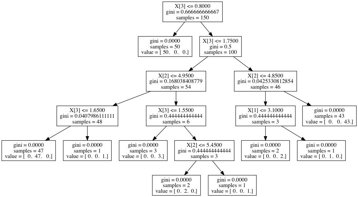
A decision tree is a binary tree which is used like a flow chart to come to a decision. At each node, one of the predictor variables is examined, and one proceeds to the left or right child based on the outcome.
Finding an optimal decision tree is NP-complete. Hence a greedy algorithm is usually used.
> install.packages('tree')
> require('tree')

> summary(iris)
  Sepal.Length    Sepal.Width     Petal.Length    Petal.Width          Species
 Min.   :4.300   Min.   :2.000   Min.   :1.000   Min.   :0.100   setosa    :50
 1st Qu.:5.100   1st Qu.:2.800   1st Qu.:1.600   1st Qu.:0.300   versicolor:50
 Median :5.800   Median :3.000   Median :4.350   Median :1.300   virginica :50
 Mean   :5.843   Mean   :3.057   Mean   :3.758   Mean   :1.199
 3rd Qu.:6.400   3rd Qu.:3.300   3rd Qu.:5.100   3rd Qu.:1.800
 Max.   :7.900   Max.   :4.400   Max.   :6.900   Max.   :2.500

> tree.iris = tree(Species~., data=iris)

> summary(tree.iris)
Classification tree:
tree(formula = Species ~ ., data = iris)
Variables actually used in tree construction:
[1] "Petal.Length" "Petal.Width"  "Sepal.Length"
Number of terminal nodes:  6
Residual mean deviance:  0.1253 = 18.05 / 144
Misclassification error rate: 0.02667 = 4 / 150

> predict(tree.iris, list(Sepal.Length=5.8, Sepal.Width=3, Petal.Length=4.35, Petal.Width=1.3))
  setosa versicolor virginica
1      0          1         0
>>> from sklearn import tree
>>> from sklearn.datasets import load_iris
>>> iris = load_iris()
>>> clf = tree.DecisionTreeClassifier()
>>> clf = clf.fit(iris.data, iris.target)
>>> from sklearn.externals.six import StringIO
>>> with open("/tmp/iris.dot", 'w') as f:
...     f = tree.export_graphviz(clf, out_file=f)
$ dot -Tpng /tmp/iris.dot > /tmp/iris.png
pruning
random forest
Decision trees tend to overfit.
Random forests use two techniques to overcome the problem. First, they use bagging, in which samples with replacement are taken repeatedly from the training data, and for each sample a decision tree is built. The final classifier takes the average of all the trees. If the response variable is categorical, the majority rule can be used.
Second, at each node of the tree, a random subset of the features is chosen as candidates for the predictor variable to be examined at that node. This is done to reduce the correlation between the trees.
> install.packages('randomForest')
> require('randomForest')
> require('MASS') # Boston

> train = sample(1:nrow(Boston), 300)
> rf.Boston = randomForest(medv ~ ., data=Boston, subset=train)
> rf.Boston

Call:
 randomForest(formula = medv ~ ., data = Boston, subset = train)
               Type of random forest: regression
                     Number of trees: 500
No. of variables tried at each split: 4

          Mean of squared residuals: 12.6554
                    % Var explained: 84.2
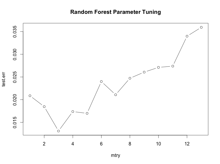
The Random Forest technique has potentially quite a few parameters, but the only one that requires tuning in practice is the number of features randomly selected at each node. If there are n features, then sqrt(n) is often a good value.
The number of trees usually doesn't have to be tuned because increasing the number of trees never results in overfitting.
Finding a good value for the number of features to randomly select:
> test.err = double(13)
> for (mtry in 1:13) {
+   fit = randomForest(medv ~ ., data=Boston, subtrain=train, mtry=mtry)
+   pred = predict(fit, Boston[-train, ])
+   test.err[mtry] = with(Boston[-train, ], mean(medv - pred)^2)
+ }
> plot(1:mtry, test.err, type='b', main='Random Forest Parameter Tuning', xlab='mtry')
>>> from sklearn.datasets import load_boston
>>> boston = load_boston()
>>> from sklearn.ensemble import RandomForestClassifier
>>> clf = RandomForestClassifier(n_estimators=400)
>>> clf = clf.fit(boston.data, boston.target)
>>> clf.predict(boston.data[0,:])
array([ 24.])
boosting
neural network
xor, parity
data sets
http://yann.lecun.com/exdb/mnist/
http://archive.ics.uci.edu/ml/datasets.html
cross validation
The test error can be used to select the best of several models, or to select a value for model with a tune-able parameter.
One technique is to split the data into two parts: training set and a validation set. Using 70% for training and 30% for validation is a popular choice. For each model, train on the training set and use the validation set to compute the test error.
Cross validation can be used to reduce the variance of the test error at the expense of training more models. The technique is to split the data into k equally sized parts. Train each model k on k - 1 of the parts, holding a different part out for computing the test error each time. The final mean-squared error is the average of the k values. k is often 5 or 10.
more topics
- measurement: accuracy, recall, precision, confusion matrix, auc, roc curve, ...
- cross validation
- ensemble methods