implementations: microsoft excel | google spreadsheet | apple numbers
Cell References
rows and columns
Excel, Numbers, and Google Spreadsheet number rows from one: 1, 2, 3, ....
Columns are given one, two, and three letter names A, B, C, ..., Y, Z, AA, AB, AC, ..., ZY, ZZ, AAA, AAB, AAC, ... The column naming scheme imposes a limit of [[$ 26 + 26^2 + 26^3 = 18,278$]] columns on a spreadsheet.
Since Numbers supports more than 18278 columns it presumably also uses column names of the form AAAA, AAAB, ....
cells
A cell is referenced by its column and row: e.g. B7. When the contents of a cell are copied to a new cell, any cell references it contains are modified by the offset between the target and source cell. This can be prevent with the dollar sign: $B7 to prevent the column from being changed, B$7 to prevent the row from being changed, and $B$7 to prevent either from being changed.
multiple sheets
If an Excel workbook has two sheets: Sheet1 and Sheet2, then a cell in Sheet2 can refer to a cell in Sheet1 with the notation
Sheet1!A1
Google Spreadsheets uses the same notation as Excel.
A Numbers sheet can have more than one table in it. The notation for referring to a cell from Sheet2 is thus:
Sheet1::Table1::A1
spreadsheet size limits
| excel (2011) | google spreadsheet | numbers | |
|---|---|---|---|
| cells | 1,048,576 * 16,384 | 200,000 | none |
| rows | 1,048,576 | 200,000 / 256 | none |
| columns | 16,384 | 256 | none |
the dependency graph
If a cell contains a reference to another cell, then it depends on that cell. If the other cell is updated, then the dependent cell is immediately updated as well. If the user introduces a cycle in the dependency graph then it is not possible for the spreadsheet to calculate the values of the cells in the cycle. The simplest example of a cycle would be to set A0 to =B0 and B0 to =A0.
When Excel, Numbers, and Google Spreadsheet detect a cycle, they will set all the cells in the cycle to an error value.
TODO: how to transpose a sheet.
TODO: sheet organization
Cell Ranges
Rectangular regions of cells can be used as arguments to functions and operands to operators. A rectangular region of cells can also be the output of a single formula.
input:
A portion of a column can be specified with the range notation B1:B7. A portion of a row can be specified with B1:F1. An arbitrary rectangular region of cells can be specified with B1:F7.
named cell range:
A cell range can be given a name. In Excel:
Insert | Name | Define...
In Google Spreadsheet:
Data | Named Ranges...
Cell range names must start with a letter and can contain letters and numbers. It is not permitted to created a cell range name which looks like a cell reference: e.g. A1, B2, ...
output:
Excel and Google Spreadsheet support formulas which output a range of cells.
In Excel, one selects the range of cells where the output will go, types in the formula, and uses Ctrl+Shift+Enter to enter it. Failure to use Ctrl+Shift+Enter results in a #VALUE! error. The shape of the selected range of cells must match the size of the output matrix. If it is too small, some values will be lost. If it is too big, the extra values will have #N/A values written to them.
In Google Spreadsheet, one selects the upper left corner of the range of cells that the output will go and then types in the formula. Typing Enter is sufficient for entering the formula. Google Spreadsheet fills in cells by expanding down or to the right.
If you inspect the output cells in Excel, you will see that all of them have the formula in them. However, in the Google Spreadsheet output, only the upper left cell has the formula, and all the other cells contain the value that was computed for that cell.
Copying
Data or formulas can be copied from one cell to another in three ways:
- using the copy (or cut) and paste short cuts
- dragging the the lower right corner of the cell to be copied. This is called auto fill.
- double clicking the lower right corner of the cell to be copied. This is also called auto fill.
There are keyboard shortcuts for Copy, Cut, and Paste. These are Ctrl+C, Ctrl+X, and Ctrl+V on Windows and ⌘C, ⌘X, ⌘V on Mac. These functions can also be performed by selecting from the Edit menu.
When a formula containing cell references is copied, the column and row of the cell reference is incremented by the difference between the source and the target unless dollar signs are used in the cell reference.
If more than one cell was copied or cut, then the same number of cells will have values pasted into them. The selected cell when
Errors
When a cell contains a formula that results in an error, one of the error values below is put in the cell.
When error values are used as values in other formulas they generally propagate.
Error values can also be created by simply typing the value into a cell.
excel
| error | condition |
|---|---|
| #NULL! | |
| #DIV/0! | division by zero |
| #VALUE! | function didn't like one of its arguments |
| #REF! | |
| #NAME? | unrecognized function or constant name |
| #NUM! | numeric overflow |
| #N/A | error created by NA() |
google spreadsheet
| error | condition |
|---|---|
| #ERROR! | parse error |
| #NULL! | |
| #DIV/0! | |
| #VALUE! | |
| #REF! | |
| #NAME? | |
| #NUM! | |
| #N/A |
Importing and Exporting
Cutting and pasting data from an HTML table to Excel often works correctly. There will be problems if cells contain newlines, however.
In general, cutting and pasting TSV text (tab and newline delimited) into Excel works. It does not seem to work in Numbers.
A good way to export data from Excel is to use Save As... (⇧⌘S) and set the format the UTF-16 Unicode Text .txt. This exports the data in a tab delimited format. Unicode characters are handled correctly. iconv can be used to convert the file to UTF-8. The various "Windows formatted" and "MS-DOS formatted" .txt and .csv options all use 8-bit encodings. Since Excel spreadsheets can contain Unicode data they should be avoided.
Sorting
excel
Select the region that is to be sorted. If you use ⌘A when a filled cell is selected, then the largest possible rectangular region of cells with filled data will be selected. If an empty cell is selected, then ⌘A causes the entire sheet to be selected.
Then select the menu "Data | Sort..." and select the column to use for sorting from the dialog box.
Pay attention to the "my list has headers" check box.
google spreadsheet
Select the label of the column to sort by. Then pull down the "Data" menu and and choose whether to sort the sheet A->Z or Z->A.
numbers
To sort the rows by a column, right click on the column label and select "Sort Ascending" or "Sort Descending".
Filtering
Before filtering, make sure the sheet has a header.
In Excel or Google Spreadsheet, select the data range and then select
Data | Filter
The column header will acquire a drop down menu that one can use to select the values to be displayed.
If the number of distinct values is small, they will be listed and one can use checkboxes to select the desired values.
Excel also permits building expressions using relational and logical operators.
In Numbers, right click the column header and select Show More Options. One will get a pop-up window which can perform sorting, filtering, and aggregation.
Joining
The VLOOKUP function can be used to perform relation join between data in two sheets. We suppose that the data is oriented so that each row corresponds to a record. If it were columns that corresponded to records, one would use the HLOOKUP function.
Imagine that we had a sheet with numbers and their English names:
| english | |
|---|---|
| 1 | one |
| 2 | two |
| 3 | three |
| 5 | five |
In another sheet we have numbers with their Spanish names:
| spanish | |
|---|---|
| 1 | uno |
| 2 | dos |
| 3 | tres |
| 4 | quatro |
In a third sheet we can join the two sheets on the first column by putting the following in the top row and then copying the values down the columns:
| =english!A1 | =VLOOKUP(A1, english!$A$1:$B$4, 2, FALSE) | =VLOOKUP(A1, spanish!$A$1:$B$4, 2, FALSE) |
|---|---|---|
| 1 | one | uno |
| 2 | two | dos |
| 3 | three | tres |
| 5 | five | #N/A |
The fourth argument of the VLOOKUP function indicates that an exact match should be used. If TRUE, and there are no exact matches, the record with the highest value less than the lookup value will be used.
To use VLOOKUP, the join column must be first in the sheets being joined. The join columns do not need to be sorted. Be careful of leading or trailing whitespace in strings. Also the type (numeric or text) must match.
By copying the join column from the first sheet, we get a left outer join. If we had copied the join column from the second sheet, we would get a right outer join.
To get an inner join one must manually find the inner join of the two join columns. One technique is to copy the first column and do a left outer join. Sort the result by a column from the second sheet and then delete all rows which have an #N/A in that value.
To get an outer join, copy both join columns into the join sheet, one below the other. Then use Data | Advanced Filter... to and select the "Unique records only" checkbox.
Aggregation
excel:
Select the region containing the data and:
Data | Summarize with PivotTable...
The first pop-up of the wizard looks like this:
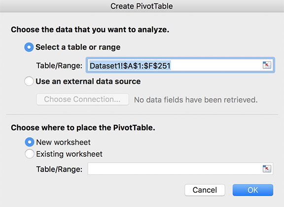
The second pop-up looks like this. Drag the fields which define the "grain" of the aggregation into the "Rows" box. Drag the fields which are going to be summed into the "Values" box.
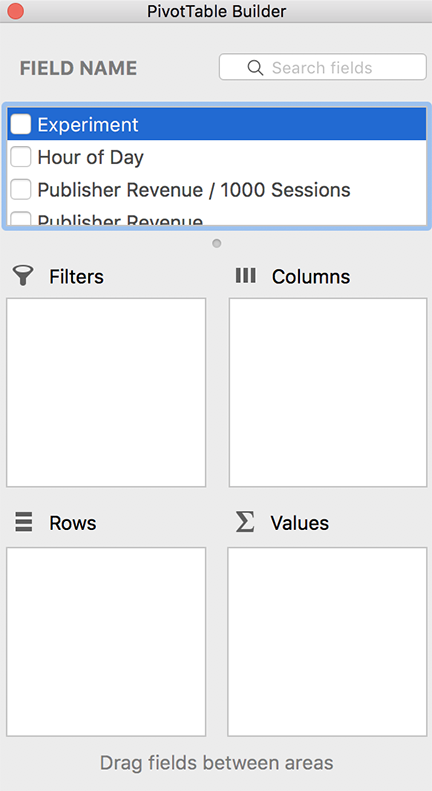
Summation is not the only aggregation function which is available. Right click on a field in the "Values" box and select "Field Settings" to change the aggregation function.
If two fields are dropped into the "Rows" box, then the data is summarized in a hierarchical manner by the first field and the combination of the first and second field.
It is also possible to the second field defining the "grain" of the aggregation into the "Columns" box. This can be nice when there is a single field in the "Values" box and putting both "grain" fields in the "Rows" box would create too many rows. Also, one gets summaries by each "grain" field in isolation.
google spreadsheet:
Data | Pivot table report...
numbers:
Right click the column header and select Categorize By This Column.
Charts
To create a chart, highlight the data region and select
Insert | Chart...
The chart is a view on the highlighted data, so if the data is changed, the chart will update itself to reflect the change.
The basic chart types are
- column
- bar
- pie
- line
- area
- scatter
column and bar charts
Column and bar charts are the same chart, except that bar charts are rotated clockwise 90°. The bar chart orientation might be useful for a chart that otherwise would be too wide to fit on a page. When a column chart is converted to a bar chart, the x-axis labels become the y-axis labels. Long text will read better on the y-axis than on the x-axis.
Column charts can be used for multivariate data, which is a range of data with more than one column. The data in each row can be stacked on top of each other or displayed side by side in clusters which are separated from other clusters by space.
If the columns and the rows have headers, these can be included in the selected range and they will be used to create labels. Row labels go on the x-axis of a column chart and the y-axis of a bar chart. Column labels go into a legend. Spreadsheets automatically detect headers if they contain text data, but one can also explicitly tell the spreadsheet to treat the first row or first column as headers.
Excel and Google Spreadsheet also have an option to make the chart treat rows as columns and columns as rows.
pie charts
A pie chart shows a univariate data set as percentages of their sum. It is a somewhat weak chart, since the data could easily be presented in a table, and experiments show that people are poor at estimating percentages from a pie chart.
Pie charts put column headers in the legend and ignore row headers.
Excel has a variant of the pie chart called the donut chart which can be used for multivariate data. Each column is represented by a concentric ring.
line charts
When the row labels are numeric, line charts are more appropriate that column charts. If no header column is selected, the labels are {1, 2, 3, ... }.
Line charts can also be used when the labels are date values, in which case the chart is a time series chart. The underlying representation of dates, i.e. days since December 31, 1899, is used.
Line charts don't seem to require that the row header be sorted. If it isn't, the data points will be plotted equidistant from each other in row order.
Column headers are put in a legend.
Line charts can be multivariate; column becomes a line in a different color.
area charts
Area charts are line charts with the area below each line filled in with a solid color.
Stack area charts are useful if the sum of each row is a meaningful quantity. For example if the columns are sales by company, then an stacked area chart will also show the total sales. It tends to be difficult, however, to read off the individual sales for companies that are not in the bottom position of the stack.
Excel has a 100% stacked area chart which can be used to show how market share changes over time. To create this type of chart in the other spreadsheets, one would have to add columns which calculate the percentages.
Google Spreadsheet, by default, uses semi-transparency for non-stacked area charts. In Excel and Numbers one can click on the area and get a popup box which allows one to adjust the opacity.
scatter plots
In Excel, the change the point marker from the default solid diamond, double click on it to get a dialog window.
In Numbers one can change the point marker in the Series pane of the Chart window.
Google Spreadsheet appears to always use solid circles, though the size and the color can be changed.
TODO: how to add another series to a scatterplot with a different color or symbol.
Linear Optimization
To solve a linear optimization problem in Excel, the Solver.Xlam add-in must be selected. Go to:
Tools | Add-Ins...
This provides a Solver button in the Data section of the ribbon.
To use it, allocate a row or column to contain the decision variables, and allocate a cell for the objective function which is defined in terms of those decision variables. The SUMPRODUCT function is useful when defining the objective function.
Click the Solver button, which brings up a dialog.
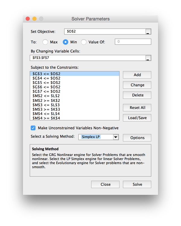
Enter the cell reference of the objective function in the topmost box.
Indicate whether the problem is a minimization or maximization problem using the radio buttons.
Enter the cell range of the decision variables in input box below that.
One enters the constaints one at a time by clicking the Add button, which brings up another dialog.
Note that there is a checkbox that can be used to indicate that all decision variables are non-negative.
User Defined Functions
- excel: visual basic module
- google spreadsheet: javascript
- numbers: doesn't have them
Notes and Presentation
- notes
- cell formats: number, alignment, font, border, fill
- column width and row height
- frozen rows and columns
To freeze a row in Mac Excel 2011, select under the bottom row to be frozen and use Window | Freeze Panes
Microsoft Excel
- can't export Unicode characters to CSV
Google Spreadsheet
Google Spreadsheets is implemented in JavaScript and runs in the browser. The spreadsheets are stored on Google's data servers. A Google spreadsheet can easily be published on the web; the document will be assigned a public URL which can be shared. It is also possible to grant read-only or read-write access to others if you know their Google email address.
- can't handle large data sets (slow with more than 2k rows)
Apple Numbers
A difference between Numbers and Excel concerns the nature of a spreadsheet. In Excel a spreadsheet is always filled with a grid of cells, but in Numbers a spreadsheet is a canvas which by default contains a single table containing a grid of cells. A Numbers canvas can contain multiple tables, or it can contain graphical items such as charts.
When a chart is created in Numbers it is placed outside of the table with the data. In Excel, by contrast, when a chart is created it floats over the spreadsheet at its grid of cells.
A Numbers table has controls at the right edge of the of the column labels and the bottom edge of the row labels to expand the size of the table by a column or a row.
- no extension language
- can't import large xlsx files (64k row limit?)
- lack of online help
- no pivot table or column grouping
- no auto fill?
- canvases with multiple tables
- export to PDF
- doesn't trim tables when exporting as CSV