Area

Measure theory attempts to extend the concepts of length, area, and volume to arbitrary subsets in ℝ, ℝ², and ℝ³. In general it attempts to assign an n-volume to arbitrary subsets of ℝⁿ.

Consider area in ℝ². The unit square is assigned an area of 1. The area of other figures is defined by how many unit squares they contain.

A rectangle with sides of length 2 and 3 can be chopped into 6 unit squares, so we get an area of 6 for the rectangle. When reasoning thus we are using finite additivity: i.e. when the sets E_j are disjoint:

We are also assuming the area of the unit square doesn't change when we move it. That is, area is invariant under translation. We also take area to be invariant under rotation and reflection.

If a rectangle has sides of length 1/2 and 1/3, we can show that has area 1/6 by chopping up the unit square into six parts of equal size.

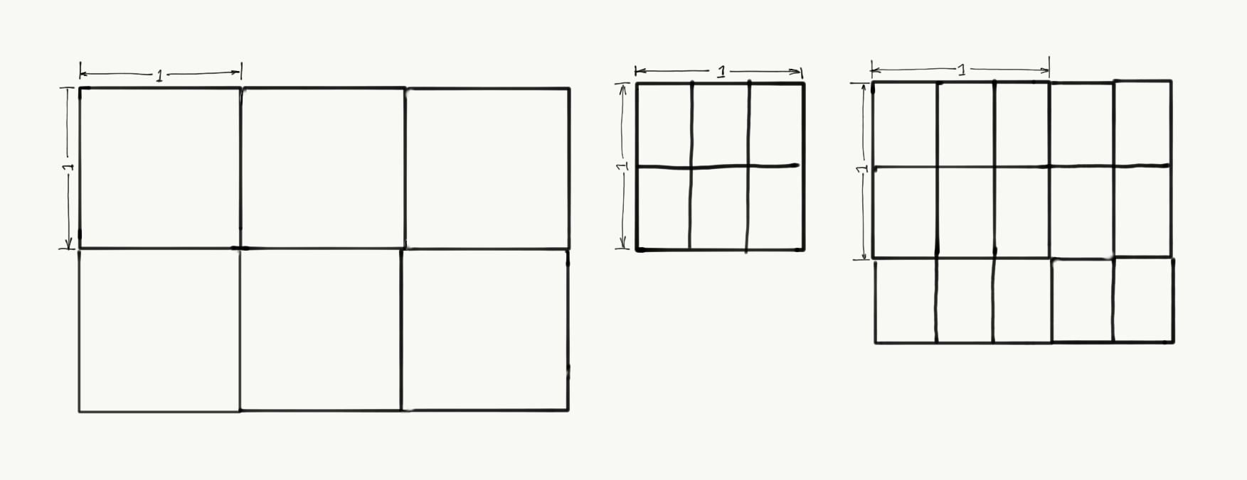
If a rectangle has sides of length 5/3 and 3/2, we can show that it has area 15/6 by chopping it into 15 rectangles with sides of length 1/2 and 1/3.

Proceeding in this fashion, we can convince ourselves that the area of a rectangle with sides of length a and b is ab, at least when a and b are rational.

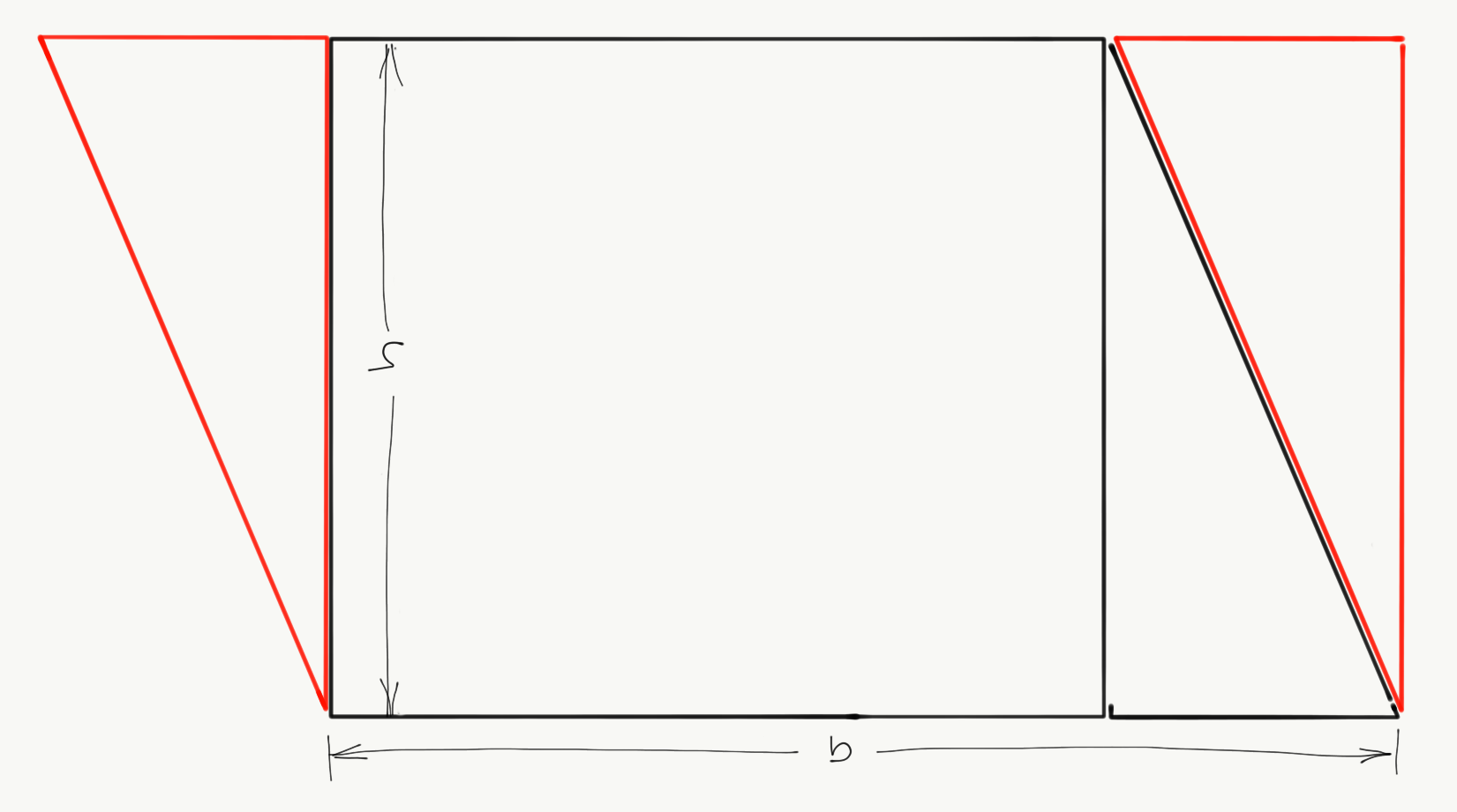
If a parallelgram has opposite sides with length b and the distance between those two sides is h, then the area is bh. We show this by chopping off a triangle from one side to "square off" one end, and translate the triangle to the other end to square it off as well, converting the parallelogram to a rectangle with equal area.

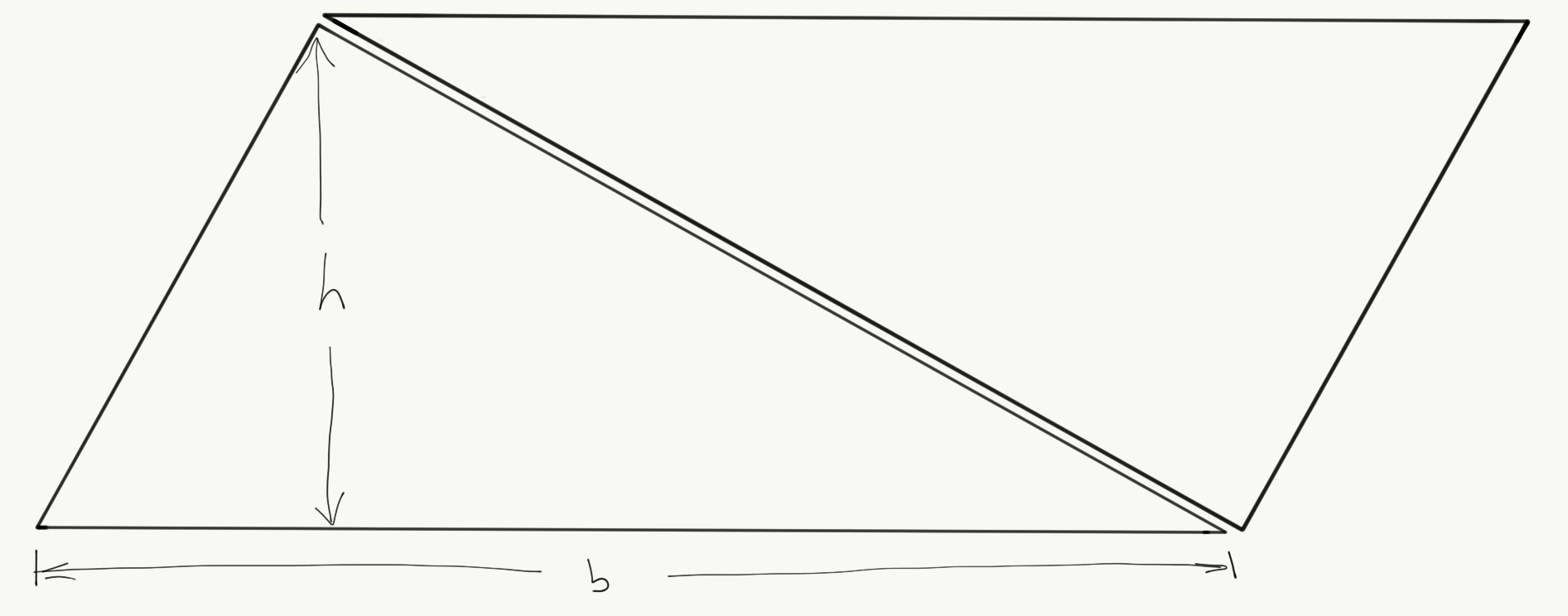
We can construct a parallelogram with twice the area of any triangle by duplicating the triangle and rotating the copy. From this we show that a triangle has area bh/2, where b is the length of one side and h is the distance from that side to the vertex not on the side.

If we know the coordinates of the vertices of a triangle, then b is easy to determine using the distance formula for two points.

h is the distance of the other vertex (x₀, y₀) to the line containing the opposite side. If the other two vertices are (x₁, y₁) and (x₂, y₂), the distance is:

Knowing the the area of a triangle, we can in principle determine the area of any region bound by a polygon with rational coordinates using polygon triangulation.

Archimedes determined the area of a circle using an infinite sequence of inscribed polygons. The technique requires a stronger condition than finite additivity, namely countable additivity. Countable additivity also allows us to extend our formulas for rectangles and triangles to figures with irrational side lengths.

The discovery of the Fundamental Theorem of Calculus in the 17th century made it possible to find the area of figures bounded by curves for which we can find the antiderivative. And even if we can't find a closed form for the antiderivative, we can integrate a Taylor series representation of the curve directly.

The proof that Isaac Barrow gave for the FTC was geometric in nature. As far as I know, the first analytic proof depended on Riemann sums and is outlined below.

A **partition** //P// of [//a//, //b//] is a finite set of points x₀, x₁, ... x_n where

We define Δx_i = x_i - x_i-1 and we also make these definitions:

The upper and lower Riemann integrals are:

If the upper and lower integrals are the same, then //f// is **Riemann integrable** on [a, b].

The FTC states that if //f// is Riemann integrable on [//a//, //b//] and if there is a differentiable function //F// on [a, b] such that F' = f, then

The proof fixes //ε// > 0 and chooses a partition //P// of [//a//, //b//] such that U(//P//, //f//) - L(//P//, //f//) < ε. It uses the MVT to find t_i
in [x_i-1, x,,i] such that

from which it follows that

Students of analysis often wonder why, after learning the Riemann integral, they must next turn their attention to the Lebesgue integral, which is conceptually more difficult. The Lebesgue integral allows us to the answer the question of which functions are Riemann integrable: those which are continuous almost everywhere. The Lebesgue integral also allows us to prove results such as the Monotone Convergence Theorem and the Dominated Convergence theorem which allow us to switch the order of integration and limits in an expression.

Definitions

• algebra
• σ-algebra
• generated σ-algebra
• Borel σ-algebra
• Borel set
• G_δ set
• F_σ set
• product σ-algebra
• elementary family
• countable additivity property
• measure
• finite measure
• σ-finite measure
• semifinite measure
• null set
• true almost everywhere
• complete measure
• outer measure
• μ^*-measurable
• premeasure
• Lebesgue-Stieltjes measure
• Lebesgue measure
• measurable function
• characteristic function
• simple function
• standard representation of a simple function
• integral of a simple function
• integral of a nonnegative function
• positive and negative parts of a function
• integral of a real valued function
• integral of a complex valued function
• Lebesgue integral
• Riemann integral
• uniform convergence
• pointwise convergence
• a.e. convergence
• Cauchy sequence in measure
• convergence in measure
• measurable rectangle
• product measure
• x-section
• y-section
• monotone class
• generated monotone class
• signed measure
• positive measure
• extended μ-integrable function
• positive set
• negative set
• null set (of a signed measure)
• Hahn decomposition
• mutually singular
• Jordan decomposition
• positive variation
• negative variation
• total variation
• finite signed measure
• σ-finite signed measure

An algebra is a set 𝒜 of subsets of X that is closed under finite unions and complements.

An σ-algebra is an algebra that is closed under countable unions.

For any set ℰ ⊆ P(X), there is a unique smallest σ-algebra containing ℰ which is called the σ-algebra generated by ℰ.

The σ-algebra generated by the open sets in a metric space or a topological space X is called the Borel σ-algebra of X and is denoted ℬ_X.

An element of a Borel σ-algebra is called a Borel set.

A countable intersection of open sets is called a G_δ set.

A countable union of closed sets is called an F_σ set.

Let {X_α}_α∈A be an indexed collection of nonempty sets, X = ∏_α∈AX_α, and π_α: X → X_α the coordinate maps. The product σ-algebra is the σ-algebra generated by

An elementary family is a collection ℰ of subsets of of X such that (1) ∅ ∈ ℰ, (2) if E, F ∈ ℰ then E ∩ F ∈ ℰ, and (3) if E ∈ ℰ then E^C is a finite disjoint union of members of ℰ.

Let X be a set with σ-algebra ℳ. A measure on (X, ℳ) is a function μ:ℳ → [0, ∞] such that (i) μ(∅) = 0 and (ii) μ has the countable additivity property, which states that if

is a sequence of disjoint sets in ℳ, then

(X, ℳ, μ) is called a measurable space, and ℳ contains the measurable sets.

//μ// is **finite** if for all //X// ∈ ℳ, //μ//(//X//) < ∞.

μ is σ-finite if for all X ∈ ℳ there exists a countable set of E_i in ℳ such that

and //μ//(//E,,i,,//) < ∞ for all E_i.

//μ// is **semifinite** if for each //E// ∈ ℳ such that //μ//(//E//) = ∞ there exists //F// ⊆ //E// such that 0 < //μ//(//F//) < ∞.

A set E such that μ(E) = 0 is called a null set.

A statement which is true for all points except those in a null set is said to be true almost everywhere.

A measure is complete if the σ-algebra contains all subsets of null sets.

An outer measure for a nonempty set X is a function μ^*: 𝒫(X) → [0, ∞] that satisfies

Let μ^* be an outer measure. A set A is μ^*-measurable if for all E ⊆ X

If 𝒜 ⊆ 𝒫(X) is an algebra, then μ₀: 𝒜 → [0, ∞] is a premeasure if

Let F: ℝ → ℝ be an increasing, right-continuous function. The Lebesgue-Stieltjes measure is the unique measure μ_F such that μ_F((a, b]) = F(b) - F(a).

The Lebesque measure is the Lebesgue-Stieltjes measure for the function F(x) = x.

If (X, ℳ) and (Y, 𝒩) are measurable spaces, then f: X → Y is (ℳ, 𝒩)-measurable if f^-1(E) ∈ ℳ for all E ∈ 𝒩.

For any E ⊆ X, the characteristic function χ_E of E is defined as

A simple function on X is a finite linear combination, with complex coefficients, of characteristic functions of sets in ℳ.

The standard representation of a simple function is the form

where E_j = f^-1({z_j}) and range(f) = {z₁, ..., z_n}.

L⁺ is the space of measurable functions from X to [0, ∞].

Let φ be a simple function in the space of measurable functions from X to [0, ∞] with standard representation

The integral of φ is:

In the above definition, the convention that 0 ⋅ ∞ = 0 is observed.

If f is any measurable function from X to [0, ∞], the integral is:

The extended real number system, [-∞, ∞], is a topological space consisting of the real numbers plus points for infinity and negative infinity.

Let f: X → [-∞, ∞]. The positive part of f is

The negative part of f is

The integral of a real valued function f is defined as

However, the integral is undefined when both ∫f⁺ and ∫f^- are infinite.

If //f// is complex valued and if ∫,,E,,|f| < ∞, then the integral of f is

The space of complex valued functions //f// for which ∫,,E,,|f| < ∞ is denoted L¹.

The Lebesgue integral is the integral as defined above when the measure is the Lebesgue measure on ℝ.

The Riemann integral...

A sequence of functions {//f//,,//n//,,} defined on //X// **converges uniformly** to //f// if for every //ε// > 0 there exists //N// such that when //n// > //N//, |//f//,,//n//,,(//x//) - //f//(//x//)| < ε for all x ∈ X.

A sequence of functions {//f//,,//n//,,} defined on //X// **converges pointwise** to //f// if for every //x// ∈ //X// and every //ε// > 0 there exists //N// which may depend on //x// such that when //n// > //N//, |//f//,,//n//,,(//x//) - //f//(//x//)| < ε.

A sequence of functions {f_n} defined on X converges a.e. to f if it converges pointwise to f for all points of X except for points in a set of measure zero.

Cauchy sequence in measure...

convergence in measure...

If (X, ℳ, μ) and (Y, 𝒩, ν) are measurable spaces, then a measurable rectangle is set in the product σ-algebra ℳ ⊗ 𝒩 of the form A × B, where A ∈ ℳ and B ∈ 𝒩.

If (X, ℳ, μ) and (Y, 𝒩, ν) are measurable spaces, then the product measure μ × ν is the restriction to ℳ ⊗ 𝒩 of the outer measure generated by the measurable rectangles of X × Y that extends the premeasure

If (X, ℳ) and (Y, 𝒩) are measurable spaces and E ⊆ X × Y, the x-section E_x is the set {y ∈ Y: (x, y) ∈ E}.

Similarly if (X, ℳ) and (Y, 𝒩) are measurable spaces and E ⊆ X × Y, the y-section E^y is the set {x ∈ X: (x, y) ∈ E}.

A monotone class on a space X is a subset 𝒞 of 𝒫(X) that is closed under countable increasing unions and countable decreasing intersections.

For any ℰ ⊆ 𝒫(X) there is a unique smallest monotone class containing ℰ, which we call the monotone class generated by ℰ.

If (X, ℳ) is a measurable space, a signed measure is a function ν: ℳ → [-∞, ∞] such that (1) ν(∅) = 0, (2) ν assumes at most of the values ±∞, and (3) if {E_j} is a sequence of disjoint sets in ℳ, then

where the latter sum converges absolutely if

is finite.

A positive measure is a signed measure with range [0, ∞]. This is a synonym for a measure.

f is an extended μ-integrable function if at least one of ∫f ⁺ dμ and ∫f ^- dμ is finite.

If ν is a signed measure on (X, ℳ), then E ∈ ℳ is a positive set if ν(F) ≥ 0 for all F ⊆ E. If ν(F) ≤ 0 or ν(F) = 0 for all F ⊆ E then E is a negative set or null set, respectively. Compare with null sets for positive measures defined previously.

The Hahn decomposition of a signed measure is the disjoint pair of sets P and N such that P ⋃ N = X, P is positive, and N is negative. The Hahn Decomposition Theorem guarantees that a Hahn decomposition exists.

Two measures μ and ν on a meaurable space (X, ℳ, μ) are mutually singular if there exist disjoint E and F such that E ⋃ F = X, E is null for μ, and F is null for ν.

The Jordan decomposition of a signed measure ν is a pair of positive measures ν⁺ and ν^- such that ν = ν⁺ - ν^- and ν⁺ ⊥ ν^-. The Jordan Decomposition Theorem guarantees that a Jordan decomposition exists.

The ν⁺ and ν^- in the Jordan decomposition of a signed measure ν are called the positive variation and negative variation of ν.

The total variation |ν| of a signed measure ν is ν⁺ + ν^- where ν⁺ and ν^- are from the Jordan decomposition. A signed measure is finite if its total variation is finite. Similarly a signed measure σ-finite if its total variation is σ-finite.

If //ν// is a signed measure and //μ// a positive measure on (//X//, ℳ), then //ν// is **absolutely continuous** with respect to //μ//, written //ν// << μ, if ν(E) = 0 for every E ∈ ℳ for which μ(E) = 0.

Lebesgue decomposition

Radon-Nikodym derivative

TODO

• Lebesgue measure
• Lebesgue integral
• Lebesgue-Stieltjes measure
• Lebesgue-Stieltjes integral
• Riemann Integral
• types of convergence
• product σ-algebras
• product measures

Theorems

Monotonicity

If (X, ℳ, μ) is a measure space, E, F ∈ ℳ, and E ⊆ F, then μ(E) ≤ μ(F).

Subadditivity

If (X, ℳ, μ) is a measure space and

then

Continuity from below

If (X, ℳ, μ) is a measure space,

and E₁ ⊆ E₂ ⊆ ⋯, then

Continuity from above

If (X, ℳ, μ) is a measure space,

and E₁ ⊇ E₂ ⊇ ⋯, then

Carathéodory's Theorem

If μ^* is an outer measure on X, the collection ℳ of μ^*-measurable sets is a σ-algebra, and the restriction of μ^* to ℳ is a complete measure.

Monotone Convergence

If {f_n} is a sequence in L⁺ such that f_j ≤ f_j+1 for all j, and

then

Fatou's Lemma

If {f_n} is any sequence in L⁺, then

Dominated Convergence Theorem

Let {f_n} be a sequence in L¹ such that (a) f_n → f a.e., and (b) there exists a nonnegative g ∈ L¹ such that |f_n| ≤ g a.e. for all n. Then f ∈ L¹ and ∫ f = lim_{n → ∞} ∫ f_n.

Egoroff's Theorem

Suppose that //μ//(//X//) < ∞ and //f//,,1,,, //f//,,2,,, ... and //f// are measurable complex-valued functions on //X// and //f//,,//n//,, → //f// a.e. Then for every //ε// > 0 there exists //E// ⊆ //X// such that //μ//(//E//) < ε and f_n → f uniformly on E^C.

Monotone Class Lemma

If 𝒜 is an algebra of subsets of X, then the monotone class 𝒞 generated by 𝒜 coincides with the σ-algebra ℳ generated by 𝒜.

Fubini-Tonelli

Suppose that (X, ℳ, μ) and (Y, 𝒩, ν) are σ-finite measure spaces.

a. (Tonelli) If f ∈ L⁺(X × Y), then the functions g(x) = ∫ f_x dν and h(y) = ∫ f^y dμ are in L⁺(X) and L⁺(Y), respectively, and

b. (Fubini) If f ∈ L¹(μ × ν), then f_x ∈ L¹(ν) for a.e. x ∈ X, f^y ∈ L¹ for a.e. y ∈ Y, the a.e.-defined functions g(x) = ∫ f_x dν and h(y) = ∫ f^ydμ are in L¹(μ) and L¹(ν), respectively, and the equations in (a) hold.

Hahn Decomposition

If ν is a signed measure on (X, ℳ), there exists a positive set P and a negative set N for ν such that P ⋃ N = X and P ⋂ N = ∅. If P', N' is another such pair, then P Δ P' (= N Δ N') is null for ν.

Jordan Decomposition

If ν is a signed measure, there exist unique positive measures ν⁺ and ν^- such that ν = ν⁺ - ν^- and ν⁺ ⊥ ν^-.

Lebesgue-Radon-Nikodym Theorem

Let ν be a σ-finite signed measure and μ a σ-finite positive measure on (X, ℳ). There exist unique σ-finite signed measures λ, ρ on (X, ℳ) such that

Moreover, there is an extended μ-integrable function f: X → ℝ such that dρ = f dμ, and any two such functions are equal μ-a.e.

Maximal

Lebesgue Differentiation

Fundamental Theorem of Calculus