Given a countable set of states, a Markov chain is a sequence of random variables X₁, X₂, X₃, ... with the Markov property: the probability of moving to the next state is independent of previous states given the present state.

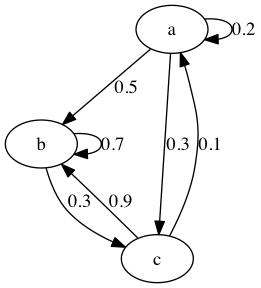
A Markov chain can be represented by a directed graph. The outgoing edges for each node should sum to 1.

Transition Matrices

If the number states is finite, we can describe the chance the process is in each state at a given time with a vector x_t of probabilities which sum to one. If we choose a column vector, then we can use a left transition matrix T—also called a left stochastic matrix—to get the chance the process is in each state at the next time. The columns of a left transition matrix sum to one.

The left transition matrix for the Markov chain depicted by the above graph is:

If row vectors are use for the state probabilities at a given time, then a right transition matrix with rows that sum to one is used to calculate state probabilities at the next time and the order of multiplication is reversed.

A Markov chain is regular if there is a positive integer n such that all entries in the transition matrix Tⁿ are positive. This is equivalent to saying that starting in any state, after n steps the process could be in the original state or any other state.

States

A state is transient if there is a non-zero probability that the process will never return to the state. Otherwise the state is said to be recurrent—or persistent.

A state is periodic with period k if the chance of returning to the state after n steps is zero when k does not divide n. The period of a state is:

An aperiodic state is a state with period 1.

A state is absorbing if a process never leaves it once it is entered.

The hitting time or return time is the amount of time it takes a process to return to a state. It can be defined as

The mean recurrence time is the expected value of the hitting time. The mean recurrence time can be infinite even if the hitting time is finite.

If the chance of eventually reaching state j from state i is greater than zero, state j is accessible from state i.

States i and j are communicating if i is accessible from j and j is accessible from i. Communication is an equivalence relation; the equivalence classes are called communicating classes. If the states in a Markov chain belong to a single communicating class, the Markov chain is irreducible.

A state is ergodic if it is aperiodic and has finite mean recurrence time.

If a Markov chain is irreducible and all its states are ergodic, then the Markov chain itself is ergodic.

Stationary Distribution

If we can represent a Markov chain by an initial state probability column vector and a single left transition matrix T, the process is said to be time homogeneous.

For such a process, a stationary distribution is a state probability vector x such that

The state probability vector is an eigenvector of the transition matrix with an eigenvalue of one. It is also a fixed point of the state transformation function.

Using MATLAB to find the stationary distribution for our example Markov chain:

>> M = [0.2 0.0 0.1; 0.5 0.7 0.9; 0.3 0.3 0.0]
M =
    0.2000         0    0.1000
    0.5000    0.7000    0.9000
    0.3000    0.3000         0

>> eig(M)
ans =
    1.0000
    0.2000
   -0.3000

>> [evecs evals] = eig(M)

>> v = evecs(:, 1) / sum(evecs(:, 1))
v =
    0.0288
    0.7404
    0.2308

>> M * v
ans =
    0.0288
    0.7404
    0.2308

A stationary distribution is not guaranteed to exist or be unique. However, an irreducible Markov chain has a stationary distribution if and only if all of its states are ergodic, and if so the stationary distribution is unique.

Markov Chain Monte Carlo (MCMC)

If a Markov Chain has a unique stationary distribution, then we can use the Markov Chain Monte Carlo method to sample from it. We choose an initial starting state x₁, and then for each state x_i we choose x_i+1 by randomly sampling according to the probabilities in the i-th column of the left transition matrix.

Here is an implementation of MCMC in Python for our example Markov chain:

$ cat mcmc.py
#!/usr/bin/env python3.5
import collections
import random

TRANSITION_MATRIX = [[0.2, 0.0, 0.1],
                     [0.5, 0.7, 0.9],
                     [0.3, 0.3, 0.0]]
BURN_IN_SIZE = 1000
SAMPLE_SIZE = 10000

def next_state(transition_matrix, state):
    val = random.random()
    so_far = 0.0
    for new_state in range(0, len(transition_matrix)):
        so_far += transition_matrix[new_state][state]
        if val <= so_far:
            return new_state

    return len(transition_matrix) - 1

def mcmc(transition_matrix, burn_in_size, sample_size):
    num_states = len(transition_matrix)
    state = random.randint(0, num_states - 1)
    state_cnt = collections.defaultdict(int)
    for _ in range(burn_in_size):
        state = next_state(transition_matrix, state)
    for _ in range(sample_size):
        state = next_state(transition_matrix, state)
        state_cnt[state] += 1
    for state in range(0, len(transition_matrix)):
        print('{}: {}'.format(state,
                              '%.3f' % (state_cnt[state] / sample_size)))

if __name__ == '__main__':
    mcmc(TRANSITION_MATRIX, BURN_IN_SIZE, SAMPLE_SIZE)

$ ./mcmc.py
0: 0.031
1: 0.740
2: 0.229

With a sample of 10,000, the algorithm was able to get two digits of accuracy.

waiting for the random walk to mix

choosing a statistic and plotting it

plotting multiple statistics from two different chains in a scatterplot

adjacent samples are usually correlated

Gibbs Sampling

Suppose that we have a Bayesian network with evidence e for the variables in E—possibly empty—and we would like to estimate the probability distribution of the remaining variables X.

Gibbs sampling is a MCMC method which can be used. Choose an order and initial values x for the variables in X. For each i in the order, we update x_i by sampling from following distribution:

Metropolis Hasting Algorithm

Let π be a distribution on the states of a Markov chain and T a transition function for the Markov chain. If following equation—the detailed balance equation—holds for all states x and x':

and if the Markov chain is regular, then π is the unique stationary distribution for T.

Suppose that have a "proposal" distribution Q(x → x') which gives the possibility of selecting the next state x' when we are at x. We want to find an "acceptance" distribution A(x → x') which either accepts the proposal—in which case the next state is x'—or rejects the proposal—in which case the next state is x—such that the detailed balance equation holds.